Image Segmentation.
图像分割 (Image Segmentation)是对图像中的每个像素进行分类,可以细分为:
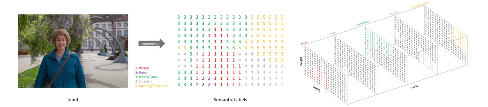
- 语义分割 (semantic segmentation):注重类别之间的区分,而不区分同一类别的不同个体;
- 实例分割 (instance segmentation):注重类别以及同一类别的不同个体之间的区分;
- 全景分割 (panoptic segmentation):对于可数的对象实例(如行人、汽车)做实例分割,对于不可数的语义区域(如天空、地面)做语义分割。

语义分割模型可以直接根据图像像素进行分组,转换为密集的分类问题。实例分割一般可分为“自上而下” 和 “自下而上”的方法,自上而下的框架是先计算实例的检测框,在检测框内进行分割;自下而上的框架则是先进行语义分割,在分割结果上对实例对象进行检测。全景分割在实例分割框架上添加语义分割分支,或基于语义分割方法采用不同的像素分组策略。本文重点关注语义分割方法。
本文目录:
- 图像分割模型
- 图像分割的评估指标
- 图像分割的损失函数
- 常用的图像分割数据集
1. 图像分割模型
图像分割的任务是使用深度学习模型处理输入图像,得到带有语义标签的相同尺寸的输出图像。
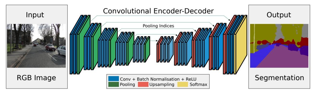
图像分割模型通常采用编码器-解码器(encoder-decoder)结构。编码器从预处理的图像数据中提取特征,解码器把特征解码为分割热图。图像分割模型的发展趋势可以大致总结为:
- 全卷积网络:FCN, SegNet, RefineNet, U-Net, V-Net, M-Net, W-Net, Y-Net, UNet++, Attention U-Net, GRUU-Net, BiSeNet V1,2, DFANet, SegNeXt
- 上下文模块:DeepLab v1,2,3,3+, PSPNet, FPN, UPerNet, EncNet, PSANet, APCNet, DMNet, OCRNet, PointRend, K-Net
- 基于Transformer:SETR, TransUNet, SegFormer, Segmenter, MaskFormer, SAM
- 通用技巧:Deep Supervision, Self-Correction
(1) 基于全卷积网络的图像分割模型
标准卷积神经网络包括卷积层、下采样层和全连接层。早期基于深度学习的图像分割模型为生成与输入图像尺寸一致的分割结果,丢弃了全连接层,并引入一系列上采样操作。因此这一阶段的模型旨在解决如何更好从卷积下采样中恢复丢掉的信息损失,逐渐形成了以U-Net为核心的对称编码器-解码器结构。
⚪ FCN
FCN提出用全卷积网络来处理语义分割问题。首先通过全卷积网络进行特征提取和下采样,然后通过双线性插值进行上采样。

⚪ SegNet
SegNet设计了对称的编码器-解码器结构,通过反池化进行上采样。
⚪ RefineNet
RefineNet把编码器产生的多个分辨率特征进行一系列卷积、融合、池化。

⚪ U-Net
U-Net使用对称的U型网络设计,在对应的下采样和上采样之间引入跳跃连接。

⚪ V-Net
V-Net是3D版本的U-Net,下采样使用步长为$2$的卷积。

⚪ M-Net
M-Net在U-Net的基础上引入了left leg和right leg。left leg使用最大池化不断下采样数据,right leg则对数据进行上采样并叠加到每一层次的输出后。

⚪ W-Net
W-Net通过堆叠两个U-Net实现无监督的图像分割。编码器U-Net提取分割表示,解码器U-Net重构原始图像。

⚪ Y-Net
Y-Net在U-Net的编码位置后增加了一个概率图预测结构,在分割任务的基础上额外引入了分类任务。

⚪ UNet++
UNet++通过跳跃连接融合了不同深度的U-Net,并为每级U-Net引入深度监督。

⚪ Attention U-Net
Attention U-Net通过引入Attention gate模块将空间注意力机制集成到U-Net的跳跃连接和上采样模块中。

⚪ GRUU-Net
GRUU-Net通过循环神经网络构造U型网络,根据多个尺度上的CNN和RNN特征聚合来细化分割结果。

⚪ BiSeNet
BiSeNet设计了一个双边结构,分别为空间路径(Spatial Path)和上下文路径(Context Path)。通过一个特征融合模块(FFM)将两个路径的特征进行融合,可以实现实时语义分割。

⚪ BiSeNet V2
BiSeNet V2精心设计了Detail Branch和Semantic Branch,使用更加轻巧的深度可分离卷积来加速模型;通过Aggregation Layer进行特征聚合;并额外引入辅助损失。

⚪ DFANet
DFANet以修改过的Xception为backbone网络,设计了一种多分支的特征重用框架来融合空间细节和上下文信息。

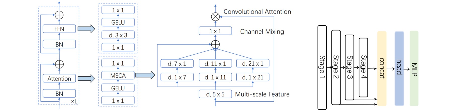
⚪ SegNeXt
SegNeXt的编码器部分采用ViT的结构,自注意力模块通过一种多尺度卷积注意力模块MSCA实现。解码器部分采用轻量型Hamberger模块对后三个阶段的特性进行聚合。
(2) 基于上下文模块的图像分割模型
多尺度问题是指当图像中的目标对象存在不同大小时,分割效果不佳的现象。比如同样的物体,在近处拍摄时物体显得大,远处拍摄时显得小。解决多尺度问题的目标就是不论目标对象是大还是小,网络都能将其分割地很好。
随着图像分割模型的效果不断提升,分割任务的主要矛盾逐渐从恢复像素信息逐渐演变为如何更有效地利用上下文(context)信息,并基于此设计了一系列用于提取多尺度特征的网络结构。
这一时期的分割网络的基本结构为:首先使用预训练模型(如ResNet)提取图像特征(通常$8 \times$下采样),然后应用精心设计的上下文模块增强多尺度特征信息,最后对特征应用上采样(通常为$8 \times$上采样)和$1\times 1$分割头生成分割结果。
有一些方法把自注意力机制引入图像分割任务,通过自注意力机制的全局交互性来捕获视觉场景中的全局依赖,并以此构造上下文模块。对于这些方法的讨论详见卷积神经网络中的自注意力机制。
⚪ Deeplab
Deeplab引入空洞卷积进行图像分割任务,并使用全连接条件随机场精细化分割结果。

⚪ DeepLab v2
Deeplab v2引入了空洞空间金字塔池化层 ASPP,即带有不同扩张率的空洞卷积的金字塔池化。

⚪ DeepLab v3
Deeplab v3对ASPP模块做了升级,把扩张率调整为$[1, 6, 12, 18]$,并增加了全局平均池化:

⚪ DeepLab v3+
Deeplab v3+采用了编码器-解码器结构。

上述Deeplab模型的对比如下:

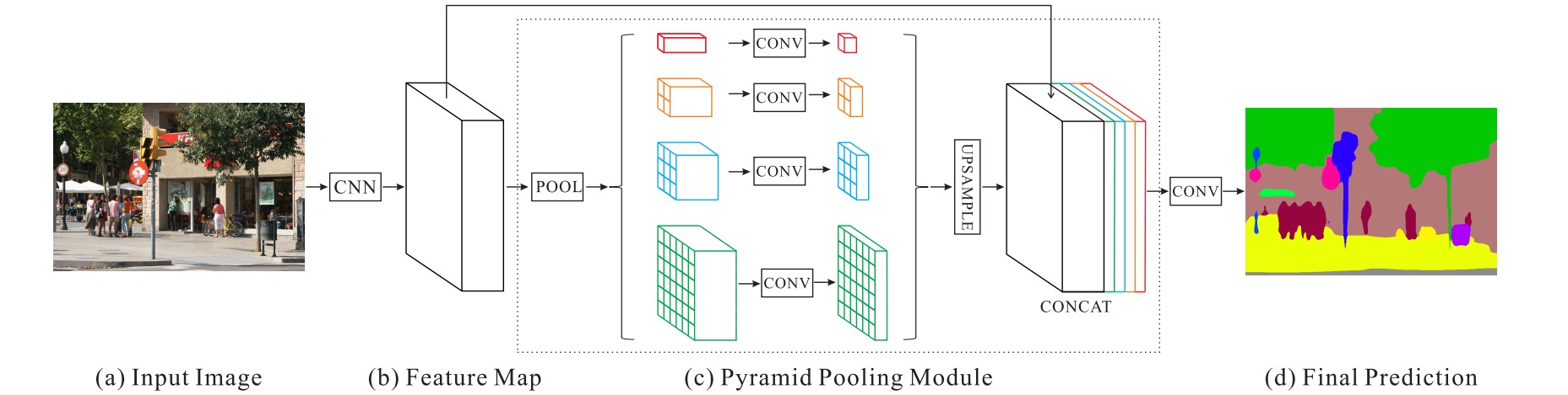
⚪ PSPNet
PSPNet引入了金字塔池化模块 PPM。PPM模块并联了四个不同大小的平均池化层,经过卷积和上采样恢复到原始大小。
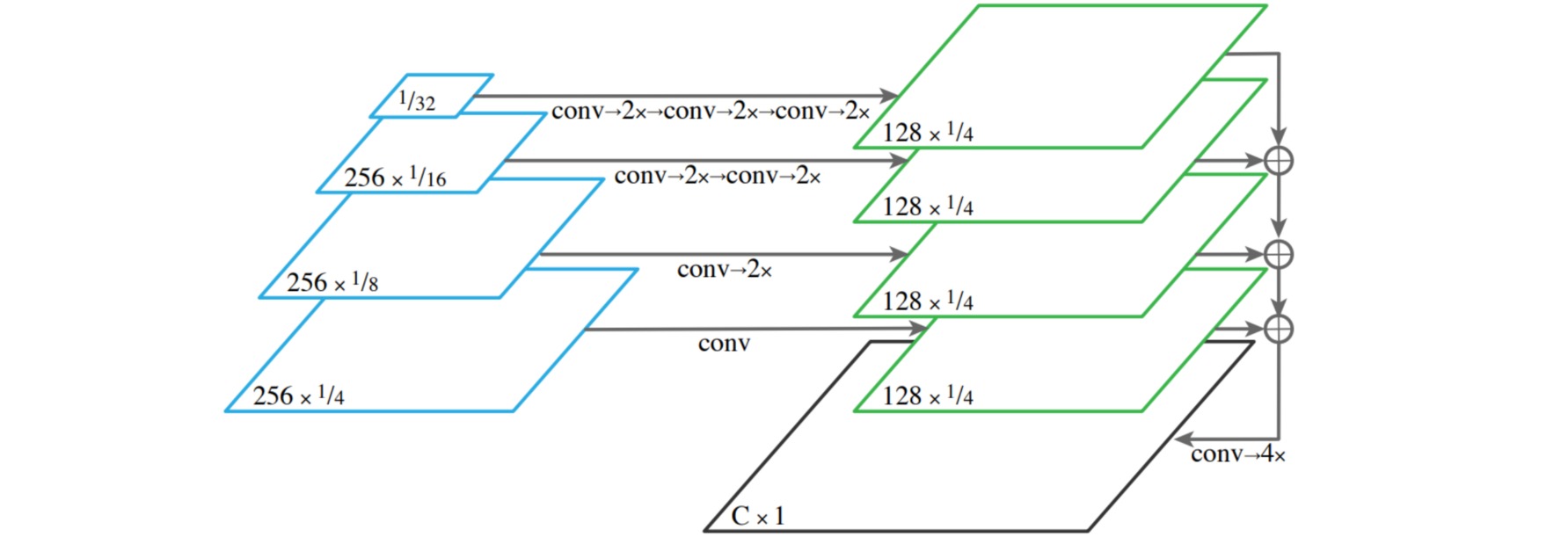
⚪ FPN
特征金字塔网络 FPN金字塔把编码器每一层的特征通过卷积和上采样合并为输出语义特征。
⚪ UPerNet
UPerNet设计了一个基于FPN和PPM的多任务分割范式,为每一个task设计了不同的检测头,可执行场景分类、目标和部位分割、材质和纹理检测。

⚪ EncNet
EncNet引入了上下文编码模块 CEM,通过字典学习和残差编码捕获全局场景上下文信息;并通过语义编码损失 SE-loss强化网络学习上下文语义。

⚪ PSANet
PSANet引入了逐点空间注意力 PSA建立每个特征像素与其他像素之间的联系,并且设计了双向的信息流传播路径。
⚪ APCNet
APCNet使用了自适应上下文模块ACM计算每个局部位置的上下文向量,并与原始特征图进行加权实现聚合上下文信息的作用。

⚪ DMNet
DMNet使用了动态卷积模块DCM来捕获多尺度语义信息,每一个DCM模块都可以处理与输入尺寸相关的比例变化。

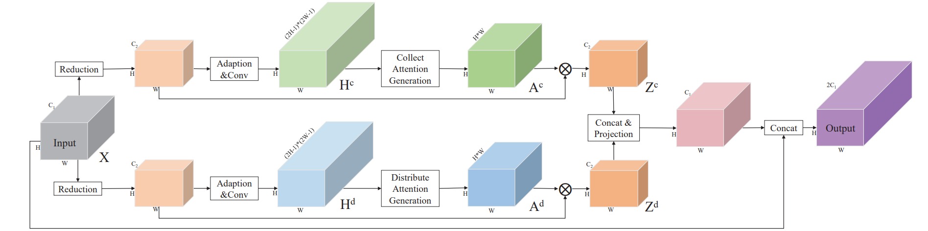
⚪ OCRNet
OCRNet根据预测结果和输出像素特征计算类别特征,然后计算像素特征与类别特征的相似度,用于增强特征的上下文表示。

⚪ PointRend
PointRend从coarse prediction中挑选N个“难点”,根据其fine-grained features和coarse prediction构造点特征向量,通过MLP网络对这些难点进行重新预测。

⚪ K-Net
K-Net提出了一种基于动态内核的分割模型,为每个任务分配不同的核来实现语义分割、实例分割和全景分割的统一。具体地,使用N个Kernel将图像划分为N组,每个Kernel都负责找到属于其相应组的像素,并应用Kernel Update Head增强Kernel的特征提取能力。

(3) 基于Transformer的图像分割模型
Transformer是一种基于自注意力机制的序列处理模型,该模型在任意层都能实现全局的感受野,建立全局依赖;而且无需进行较大程度的下采样就能实现特征提取,保留了图像的更多信息。
⚪ SETR
SETR采取了ViT作为编码器提取图像特征;通过基于卷积的渐进上采样或者多层次特征聚合生成分割结果。

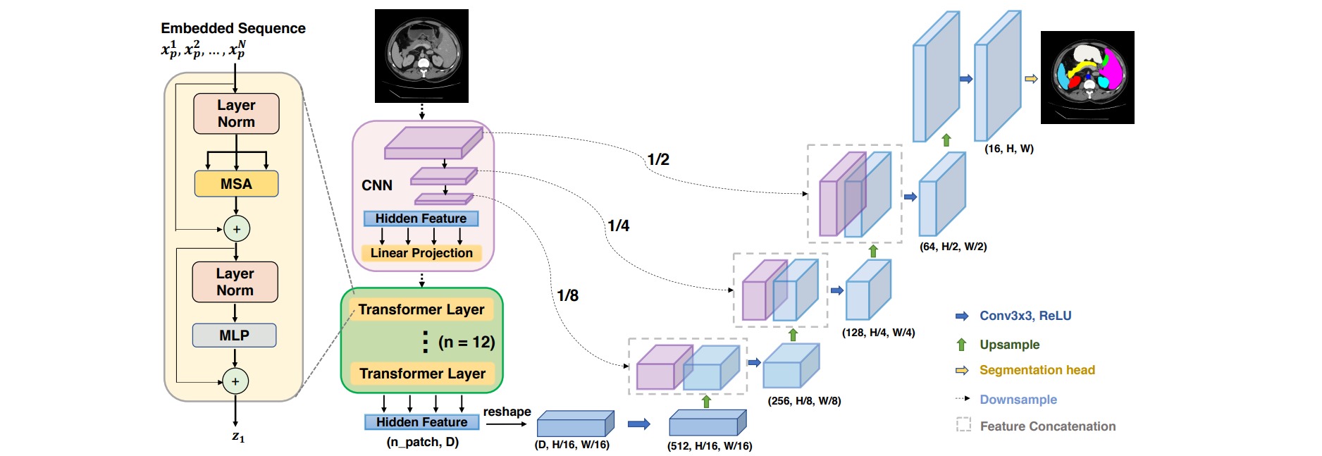
⚪ TransUNet
TransUNet的Encoder部分主要由ResNet50和ViT组成,其中前三个模块为两倍下采样的ResNet Block,最后一个模块为12层Transformer Layer。
⚪ SegFormer
SegFormer包括用于生成多尺度特征的分层Encoder(包含Efficient Self-Attention、Mix-FFN和Overlap Patch Embedding三个模块)和仅由MLP层组成的轻量级All-MLP Decoder。

⚪ Segmenter
Segmenter完全基于Transformer的编码器-解码器架构。图像块序列由Transformer编码器编码,并由mask Transformer解码。Mask Transformer引入一组个可学习的类别嵌入,通过计算其与解码序列特征的乘积来生成每个图像块的分割图。

⚪ MaskFormer
MaskFormer把分割问题看作掩码级的分类问题。对输入图像生成$N$个二值掩码,并为每个掩码预测$K+1$个类别中的某个。

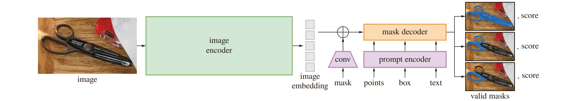
⚪ Segment Anything
SAM是一个图像分割的基础模型,模型的设计和训练是通过提示工程实现的。SAM采用一种简单的设计:一个图像编码器生成图像嵌入,一个提示编码器生成提示嵌入,然后将这两种嵌入组合后通过一个轻量级掩码解码器预测分割掩码。
(4) 分割模型中的通用技巧
⚪ Deep Supervision
深度监督(Deep Supervision)是在深度神经网络的某些隐藏层后增加一个辅助的分类器作为一种网络分支来对主干网络进行监督的技巧,用来解决深度神经网络训练梯度消失和收敛速度过慢等问题。
一个带有深度监督的八层卷积网络结构如下图所示。在Conv4之后添加了一个监督分类器作为分支。Conv4输出的特征图除了随着主网络进入Conv5之外,也作为输入进入分支分类器。

⚪ Self-Correction
- Reference:Self-Correction for Human Parsing
图像分割任务的标签可能存在噪声。自校正(Self-Correction)是一种净化分割标签噪声的方法。模型训练从具有噪声的标签出发,通过聚合当前模型和前一个最优模型的参数来推断更可靠的标签,并用这些更正的标签训练更鲁棒的模型。
自校正包括模型聚合和标签聚合两个过程。对于模型聚合,记录当前轮数的训练权重$\hat{w}$与之前训练的最优权重$\hat{w}_{m-1}$,得到融合权重并更新历史最优权重:
\[\hat{w}_m = \frac{m}{m+1}\hat{w}_{m-1} + \frac{1}{m+1}\hat{w}\]标签的更新类似,通过融合当前预测结果$\hat{y}$和前一轮标签$\hat{y}_{m-1}$获得类别关系更明确的新标签:
\[\hat{y}_m = \frac{m}{m+1}\hat{y}_{m-1} + \frac{1}{m+1}\hat{y}\]
⭐ 参考文献
- Fully Convolutional Networks for Semantic Segmentation:(arXiv1411)FCN: 语义分割的全卷积网络。
- Semantic Image Segmentation with Deep Convolutional Nets and Fully Connected CRFs:(arXiv1412)DeepLab: 通过深度卷积网络和全连接条件随机场实现图像语义分割。
- U-Net: Convolutional Networks for Biomedical Image Segmentation:(arXiv1505)U-Net: 用于医学图像分割的卷积网络。
- SegNet: A Deep Convolutional Encoder-Decoder Architecture for Image Segmentation:(arXiv1511)SegNet: 图像分割的深度卷积编码器-解码器结构。
- V-Net: Fully Convolutional Neural Networks for Volumetric Medical Image Segmentation:(arXiv1606)V-Net:用于三维医学图像分割的全卷积网络。
- DeepLab: Semantic Image Segmentation with Deep Convolutional Nets, Atrous Convolution, and Fully Connected CRFs:(arXiv1606)DeepLab v2: 通过带有空洞卷积的金字塔池化实现图像语义分割。
- RefineNet: Multi-Path Refinement Networks for High-Resolution Semantic Segmentation:(arXiv1611)RefineNet: 高分辨率语义分割的多路径优化网络。
- Pyramid Scene Parsing Network:(arXiv1612)PSPNet: 金字塔场景解析网络。
- M-Net: A Convolutional Neural Network for Deep Brain Structure Segmentation:(ISBI 2017)M-Net:用于三维脑结构分割的二维卷积神经网络。
- Rethinking Atrous Convolution for Semantic Image Segmentation:(arXiv1706)DeepLab v3: 重新评估图像语义分割中的扩张卷积。
- W-Net: A Deep Model for Fully Unsupervised Image Segmentation:(arXiv1711)W-Net:一种无监督的图像分割方法。
- Encoder-Decoder with Atrous Separable Convolution for Semantic Image Segmentation:(arXiv1802)DeepLab v3+: 图像语义分割中的扩张可分离卷积。
- Context Encoding for Semantic Segmentation:(arXiv1803)EncNet: 语义分割的上下文编码。
- Attention U-Net: Learning Where to Look for the Pancreas:(arXiv1804)Attention U-Net: 向U-Net引入注意力机制。
- Y-Net: Joint Segmentation and Classification for Diagnosis of Breast Biopsy Images:(arXiv1806)Y-Net:乳腺活检图像的分割和分类。
- UNet++: A Nested U-Net Architecture for Medical Image Segmentation:(arXiv1807)UNet++:用于医学图像分割的巢型UNet。
- Unified Perceptual Parsing for Scene Understanding:(arXiv1807)UPerNet: 场景理解的统一感知解析。
- BiSeNet: Bilateral Segmentation Network for Real-time Semantic Segmentation:(arXiv1808)BiSeNet: 实时语义分割的双边分割网络。
- PSANet: Point-wise Spatial Attention Network for Scene Parsing:(ECCV2018)PSANet: 场景解析的逐点空间注意力网络。
- GRUU-Net: Integrated convolutional and gated recurrent neural network for cell segmentation:(Medical Image Analysis2018)GRUU-Net: 细胞分割的融合卷积门控循环神经网络。
- Panoptic Feature Pyramid Networks:(arXiv1901)全景特征金字塔网络。
- DFANet: Deep Feature Aggregation for Real-Time Semantic Segmentation:(arXiv1904)DFANet: 实时语义分割的深度特征聚合。
- Object-Contextual Representations for Semantic Segmentation:(arXiv1909)OCRNet:语义分割中的目标上下文表示。
- PointRend: Image Segmentation as Rendering:(arXiv1912)PointRend: 把图像分割建模为渲染。
- Adaptive Pyramid Context Network for Semantic Segmentation:(CVPR2019)APCNet: 语义分割的自适应金字塔上下文网络。
- Dynamic Multi-Scale Filters for Semantic Segmentation:(ICCV2019)DMNet: 语义分割的动态多尺度滤波器。
- BiSeNet V2: Bilateral Network with Guided Aggregation for Real-time Semantic Segmentation:(arXiv2004)BiSeNet V2: 实时语义分割的带引导聚合的双边网络。
- Rethinking Semantic Segmentation from a Sequence-to-Sequence Perspective with Transformers:(arXiv2012)用Transformer从序列到序列的角度重新思考语义分割。
- TransUNet: Transformers Make Strong Encoders for Medical Image Segmentation:(arXiv2102)TransUNet:用Transformer为医学图像分割构造强力编码器。
- SegFormer: Simple and Efficient Design for Semantic Segmentation with Transformers:(arXiv2105)SegFormer:为语义分割设计的简单高效的Transformer模型。
- Segmenter: Transformer for Semantic Segmentation:(arXiv2105)Segmenter:为语义分割设计的视觉Transformer。
- K-Net: Towards Unified Image Segmentation:(arXiv2106)K-Net: 面向统一的图像分割。
- Per-Pixel Classification is Not All You Needfor Semantic Segmentation:(arXiv2107)MaskFormer:逐像素分类并不是语义分割所必需的。
- SegNeXt: Rethinking Convolutional Attention Design for Semantic Segmentation:(arXiv2209)SegNeXt:重新思考语义分割中的卷积注意力设计。
- Segment Anything:(arXiv2304)SAM:分割任意模型。
2. 图像分割的评估指标
图像分割任务本质上是一种图像像素分类任务,可以使用常见的分类评价指标来评估模型的好坏。图像分割中常用的评估指标包括:
- 像素准确率 (pixel accuracy, PA)
- 类别像素准确率 (class pixel accuracy, CPA)
- 类别平均像素准确率 (mean pixel accuracy, MPA)
- 交并比 (Intersection over Union, IoU)
- 平均交并比 (mean Intersection over Union, MIoU)
- 频率加权交并比 (Frequency Weighted Intersection over Union, FWIoU)
- Dice系数 (Dice Coefficient)
上述评估指标均建立在混淆矩阵的基础之上,因此首先介绍混淆矩阵,然后介绍这些评估指标的计算。
⚪ 混淆矩阵
图像分割问题本质上是对图像中的像素的分类问题。
(1) 二分类
以二分类为例,图像中的每个像素可能属于正例(Positive)也可能属于反例(Negative)。根据像素的实际类别和模型的预测结果,可以把像素划分为以下四类中的某一类:
- 真正例 TP(True Positive):实际为正例,预测为正例
- 假正例 FP(False Positive):实际为反例,预测为正例
- 真反例 TN(True Negative):实际为反例,预测为反例
- 假反例 FN(False Negative):实际为正例,预测为反例
绘制分类结果的混淆矩阵(confusion matrix)如下:
\[\begin{array}{l|cc} \text{真实情况\预测结果} & \text{正例} & \text{反例} \\ \hline \text{正例} & TP & FN \\ \text{反例} & FP & TN \\ \end{array}\]根据混淆矩阵可做如下计算:
- 准确率(accuracy),定义为模型分类正确的像素比例:
- 查准率(precision),定义为模型预测为正例的所有像素中,真正为正例的像素比例:
- 查全率(recall),又称召回率,定义为所有真正为正例的像素中,模型预测为正例的像素比例:
- F1分数(F1-Score),定义为查准率和召回率的调和平均数。
(2) 多分类
图像分割通常是多分类问题,也有类似结论。对于多分类问题,混淆矩阵表示如下:
\[\begin{array}{l|ccc} \text{真实情况\预测结果} & \text{类别1} & \text{类别2} & \text{类别3} \\ \hline \text{类别1} & a & b & c \\ \text{类别2} & d & e & f \\ \text{类别3} & g & h & i \\ \end{array}\]对于多分类问题,也可计算:
- 准确率:
- 查准率,以类别$1$为例:
- 查全率,以类别$1$为例:
(3) 计算混淆矩阵
对于图像分割的预测结果imgPredict和真实标签imgLabel,可以使用np.bincount函数计算混淆矩阵,计算过程如下:
import numpy as np

def genConfusionMatrix(numClass, imgPredict, imgLabel):
    '''
    Parameters
    ----------
    numClass : 类别数(不包括背景).
    imgPredict : 预测图像.
    imgLabel : 标签图像.
    '''
    # remove classes from unlabeled pixels in gt image and predict
    mask = (imgLabel >= 0) & (imgLabel < numClass)

    label = numClass * imgLabel[mask] + imgPredict[mask]
    count = np.bincount(label, minlength=numClass**2)
    confusionMatrix = count.reshape(numClass, numClass)
    return confusionMatrix

imgPredict = np.array([[0,1,0],
                 [2,1,0],
                 [2,2,1]])
imgLabel = np.array([[0,2,0],
                  [2,1,0],
                  [0,2,1]])
print(genConfusionMatrix(3, imgPredict, imgLabel))

###
[[3 0 1]
 [0 2 0]
 [0 1 2]]
###
⚪ 像素准确率 PA
像素准确率 (pixel accuracy, PA) 衡量所有类别预测正确的像素占总像素数的比例,相当于分类任务中的准确率(accuracy)。
PA计算为混淆矩阵对角线元素之和比矩阵所有元素之和,以二分类为例:
\[\text{PA} = \frac{TP+TN}{TP+FP+TN+FN}\]def pixelAccuracy(confusionMatrix):
# return all class overall pixel accuracy
# PA = acc = (TP + TN) / (TP + TN + FP + TN)
acc = np.diag(confusionMatrix).sum() / confusionMatrix.sum()
return acc
⚪ 类别像素准确率 CPA
类别像素准确率 (class pixel accuracy, CPA) 衡量在所有预测类别为$i$的像素中,真正属于类别$i$的像素占总像素数的比例,相当于分类任务中的查准率(precision)。
第$i$个类别的CPA计算为混淆矩阵第$i$个对角线元素比矩阵该列元素之和。以二分类为例,第$0$个类别的CPA计算为:
\[\text{CPA} = \frac{TP}{TP+FP}\]def classPixelAccuracy(confusionMatrix):
# return each category pixel accuracy(A more accurate way to call it precision)
# acc = (TP) / TP + FP
classAcc = np.diag(confusionMatrix) / confusionMatrix.sum(axis=0)
return classAcc # 返回一个列表,表示各类别的预测准确率
⚪ 类别平均像素准确率 MPA
类别平均像素准确率 (mean pixel accuracy, MPA) 计算为所有类别的CPA的平均值:
\[\text{MPA} = \text{mean}(\text{CPA})\]def meanPixelAccuracy(confusionMatrix):
classAcc = classPixelAccuracy(confusionMatrix)
meanAcc = np.nanmean(classAcc) # np.nanmean表示遇到Nan类型,其值取为0
return meanAcc
⚪ 交并比 IoU
交并比 (Intersection over Union, IoU) 又称Jaccard index,衡量预测类别为$i$的像素集合$A$和真实类别为$i$的像素集合$B$的交集与并集之比。
\[\text{IoU} = \frac{|A ∩ B |}{|A ∪ B|}= \frac{|A ∩ B |}{|A|+| B |-|A ∩ B |}\]预测类别为$i$的像素集合是指所有预测为类别$i$的像素,用混淆矩阵第$i$列元素之和表示。真实类别为$i$的像素集合是指所有实际类别$i$的像素,用混淆矩阵第$i$行元素之和表示。
第$i$个类别的IoU计算为混淆矩阵第$i$个对角线元素比矩阵该列元素与该行元素的并集。以二分类为例,第$0$个类别的IoU计算为:
\[\text{IoU} = \frac{TP}{TP+FP+FN}\]def IntersectionOverUnion(confusionMatrix):
# Intersection = TP Union = TP + FP + FN
# IoU = TP / (TP + FP + FN)
intersection = np.diag(confusionMatrix)
union = np.sum(confusionMatrix, axis=1) + np.sum(confusionMatrix, axis=0) - np.diag(confusionMatrix)
IoU = intersection / union
return IoU # 返回列表,其值为各个类别的IoU
⚪ 平均交并比 MIoU
平均交并比 (mean Intersection over Union, MIoU) 计算为所有类别的IoU的平均值:
\[\text{MIoU} = \text{mean}(\text{IoU})\]def meanIntersectionOverUnion(confusionMatrix):
IoU = IntersectionOverUnion(confusionMatrix)
mIoU = np.nanmean(IoU) # 求各类别IoU的平均
return mIoU
⚪ 频率加权交并比 FWIoU
频率加权交并比 (Frequency Weighted Intersection over Union, FWIoU) 按照真实类别为$i$对应像素占所有像素的比例对类别$i$的IoU进行加权。
第$i$个类别的FWIoU首先计算混淆矩阵第$i$行元素求和比矩阵所有元素求和,再乘以第$i$个类别的IoU。以二分类为例,第$0$个类别的FWIoU计算为:
\[\text{FWIoU} = \frac{TP+FN}{TP+FP+FN+TN} \cdot \frac{TP}{TP+FP+FN}\]最终给出的FWIoU应为所有类别FWIoU的求和。
def Frequency_Weighted_Intersection_over_Union(confusion_matrix):
    # FWIOU = [(TP+FN)/(TP+FP+TN+FN)] *[TP / (TP + FP + FN)]
    freq = np.sum(confusion_matrix, axis=1) / np.sum(confusion_matrix)
    iu = np.diag(confusion_matrix) / (
            np.sum(confusion_matrix, axis=1) +
            np.sum(confusion_matrix, axis=0) -
            np.diag(confusion_matrix))
    FWIoU = (freq[freq > 0] * iu[freq > 0]).sum()
    return FWIoU
⚪ Dice Coefficient
Dice Coefficient衡量预测类别为$i$的像素集合$A$和真实类别为$i$的像素集合$B$之间的相似程度。
预测类别为$i$的像素集合是指所有预测为类别$i$的像素,用混淆矩阵第$i$列元素之和表示。真实类别为$i$的像素集合是指所有实际类别$i$的像素,用混淆矩阵第$i$行元素之和表示。
Dice Coefficient的计算相当于IoU的分子分母同时加上两个集合的交集。
\[\text{Dice} = \frac{2|A ∩ B |}{|A|+| B |} = \frac{2\text{IoU}}{1+\text{IoU}}\]第$i$个类别的Dice计算为混淆矩阵第$i$个对角线元素的两倍比矩阵该列元素与该行元素之和。以二分类为例,第$0$个类别的Dice计算为:
\[\text{Dice} = \frac{2TP}{2TP+FP+FN} = \text{F1-score}\]因此Dice系数等价于分类指标中的F1-Score。
def Dice(confusionMatrix):
    # Dice = 2*TP / (TP + FP + TP + FN)
    intersection = np.diag(confusionMatrix)
    Dice = 2*intersection / (
        np.sum(confusionMatrix, axis=1) + np.sum(confusionMatrix, axis=0))
    return Dice # 返回列表,其值为各个类别的Dice
特别地,对于二值分割问题,Dice系数可以直接通过\(\{0,1\}\)预测矩阵和标签矩阵计算:
def dice_coef(pred, target):
    """
    Dice =  2*sum(|A*B|)/(sum(A^2)+sum(B^2))
    """
    smooth = 1.
    m1 = pred.view(-1).float()
    m2 = target.view(-1).float()
    intersection = (m1 * m2).sum().float()
    dice = (2. * intersection + smooth) / (torch.sum(m1*m1) + torch.sum(m2*m2) + smooth)
    return dice
3. 图像分割的损失函数
本节参考论文 Loss odyssey in medical image segmentation 和Github库 SegLoss: A collection of loss functions for medical image segmentation。
图像分割的损失函数用于衡量预测分割结果和真实标签之间的差异。一个合理的损失函数不仅用于指导网络学习在给定评估指标上与真实标签相接近的预测结果,还启发网络如何权衡错误结果(如假阳性、假阴性)。
根据损失函数的推导方式不同,图像分割任务中常用的损失函数可以划分为:
- 基于分布的损失:Cross-Entropy Loss, Weighted Cross-Entropy Loss, TopK Loss, Focal Loss, Distance Map Penalized CE Loss
- 基于区域的损失:Sensitivity-Specifity Loss, IoU Loss, Lovász Loss, Dice Loss, Tversky Loss, Focal Tversky Loss, Asymmetric Similarity Loss, Generalized Dice Loss, Penalty Loss,
- 基于边界的损失:Boundary Loss, Hausdorff Distance Loss
在实践中,通常使用上述损失函数的组合形式,如Cross-Entropy Loss + Dice Loss。

(1) 基于分布的损失 Distribution-based Loss
基于分布的损失函数旨在最小化两种分布之间的差异。
⚪ Cross-Entropy Loss
交叉熵损失是由KL散度导出的,衡量数据分布$P$和预测分布$Q$之间的差异:
\[\begin{aligned} D_{K L}(P \mid Q) & =\sum_i p_i \log \frac{p_i}{q_i} \\ & =-\sum_i p_i \log q_i+\sum_i p_i \log p_i \\ & =H(P, Q)-H(P) \end{aligned}\]注意到数据分布$P$通常是已知的,因此最小化数据分布$P$和预测分布$Q$之间的KL散度等价于最小化交叉熵$H(P,Q)$。对于分割任务,指定$g_i^c$是像素$i$是否属于标签$c$的二元指示符,$s_i^c$是对应的预测结果,则交叉熵损失定义为:
\[L_{C E}=-\frac{1}{N} \sum_{c=1}^C \sum_{i=1}^N g_i^c \log s_i^c\]ce_loss = torch.nn.CrossEntropyLoss()
# result无需经过Softmax,gt为整型
loss = ce_loss(result, gt)
⚪ Weighted Cross-Entropy Loss
为缓解类别不平衡问题,加权交叉熵损失为每个类别指定一个权重$w_c$。权重$w_c$通常与类别出现频率成反比,比如设置为训练集中类别出现频率的倒数。
\[L_{W C E}=-\frac{1}{N} \sum_{c=1}^c \sum_{i=1}^N w_c g_i^c \log s_i^c\]wce_loss = torch.nn.CrossEntropyLoss(weight=weight)
loss = wce_loss(result, gt)
⚪ TopK Loss
TopK损失旨在迫使网络在训练过程中专注于难例样本(hard samples)。在计算交叉熵损失时,只保留前$k\%$个最差的(损失最大的)分类像素。
\[L_{\text {Top} K}=-\frac{1}{N} \sum_{c=1}^c \sum_{i \in \mathbf{K}} g_i^c \log s_i^c\]class TopKLoss(nn.Module):
def __init__(self, weight=None, ignore_index=-100, k=10):
super(TopKLoss, self).__init__()
self.k = k
self.ce_loss = torch.nn.CrossEntropyLoss(reduce=False)
def forward(self, result, gt):
res = self.ce_loss(result, gt)
num_pixels = np.prod(res.shape)
res, _ = torch.topk(res.view((-1, )), int(num_pixels * self.k / 100), sorted=False)
return res.mean()
⚪ Focal Loss
Focal Loss通过减少容易分类像素的损失权重,以处理前景-背景类别的不平衡问题。
\[L_{\text {Focal }}=-\frac{1}{N} \sum_c^c \sum_{i=1}^N\left(1-s_i^c\right)^\gamma g_i^c \log s_i^c\]from einops import rearrange
class FocalLoss(nn.Module):
def __init__(self, gamma=2):
super(FocalLoss, self).__init__()
self.gamma = gamma
def forward(self, result, gt):
result = rearrange(result, 'b c h w -> b c (h w)')
result = torch.softmax(result, dim=1)
gt = rearrange(gt, 'b h w -> b 1 (h w)')
y_onehot = torch.zeros_like(result)
y_onehot = y_onehot.scatter_(1, gt.data, 1)
pt = (y_onehot * result).sum(1)
logpt = pt.log()
gamma = self.gamma
loss = -1 * torch.pow((1 - pt), gamma) * logpt
return loss.mean()
⚪ Distance Map Penalized CE Loss
距离图惩罚交叉熵损失通过由真实标签计算的距离变换图对交叉熵进行加权,引导网络重点关注难以分割的边界区域。
\[L_{D P C E}=-\frac{1}{N} \sum_{c=1}^c\left(1+D^c\right) \circ \sum_{i=1}^N g_i^c \log s_i^c\]其中$D^c$是类别$c$的距离惩罚项,通过取真实标签的距离变换图的倒数来生成。通过这种方式可以为边界上的像素分配更大的权重。
from einops import rearrange
from scipy.ndimage import distance_transform_edt

class DisPenalizedCE(torch.nn.Module):
    def __init__(self):
        super(DisPenalizedCE, self).__init__()

    @torch.no_grad()
    def one_hot2dist(self, seg):
        res = np.zeros_like(seg)
        for c in range(seg.shape[1]):
            posmask = seg[:,c,...]
            if posmask.any():
                negmask = 1.-posmask
                pos_edt = distance_transform_edt(posmask)
                pos_edt = (np.max(pos_edt)-pos_edt)*posmask
                neg_edt =  distance_transform_edt(negmask)
                neg_edt = (np.max(neg_edt)-neg_edt)*negmask
                res[:,c,...] = pos_edt + neg_edt
        return res

    def forward(self, result, gt):
        result = torch.softmax(result, dim=1)
        gt = rearrange(gt, 'b h w -> b 1 h w')

        y_onehot = torch.zeros_like(result)
        y_onehot = y_onehot.scatter_(1, gt.data, 1)
        dist = torch.from_numpy(self.one_hot2dist(y_onehot.cpu().numpy())+1).float()

        result = torch.softmax(result, dim=1)
        result_logs = torch.log(result)

        loss = -result_logs * y_onehot
        weighted_loss = loss*dist
        return weighted_loss.mean()
(2) 基于区域的损失 Region-based Loss
基于区域的损失函数旨在最小化真实标签$G$和预测分割$S$之间的不匹配程度或者最大化两者之间的重叠区域。
⚪ Sensitivity-Specifity Loss
敏感性-特异性损失通过加权敏感性与特异性来解决类别不平衡问题:
\[\begin{aligned} L_{S S}= & w \frac{\sum_{c=1}^C \sum_{i=1}^N\left(g_i^c-s_i^c\right)^2 g_i^c}{\sum_{c=1}^C \sum_{i=1}^N g_i^c+\epsilon} \\ & +(1-w) \frac{\sum_{c=1}^C \sum_{i=1}^N\left(g_i^c-s_i^c\right)^2\left(1-g_i^c\right)}{\sum_{c=1}^C \sum_{i=1}^N\left(1-g_i^C\right)+\epsilon} \end{aligned}\]from einops import rearrange, einsum
class SSLoss(nn.Module):
def __init__(self, smooth=1.):
super(SSLoss, self).__init__()
self.smooth = smooth
self.r = 0.1 # weight parameter in SS paper
def forward(self, result, gt):
result = rearrange(result, 'b c h w -> b c (h w)')
result = torch.softmax(result, dim=1)
gt = rearrange(gt, 'b h w -> b 1 (h w)')
y_onehot = torch.zeros_like(result)
y_onehot = y_onehot.scatter_(1, gt.data, 1)
# no object value
bg_onehot = 1 - y_onehot
squared_error = (y_onehot - result)**2
specificity_numerator = einsum(squared_error, y_onehot, 'b c n, b c n -> b c')
specificity_denominator = einsum(y_onehot, 'b c n -> b c')+self.smooth
specificity_part = einsum(specificity_numerator, 'b c -> b')/einsum(specificity_denominator, 'b c -> b')
sensitivity_numerator = einsum(squared_error, bg_onehot, 'b c n, b c n -> b c')
sensitivity_denominator = einsum(bg_onehot, 'b c n -> b c')+self.smooth
sensitivity_part = einsum(sensitivity_numerator, 'b c -> b')/einsum(sensitivity_denominator, 'b c -> b')
ss = self.r * specificity_part + (1-self.r) * sensitivity_part
return ss.mean()
⚪ IoU Loss
IoU Loss直接优化IoU index。由于预测热图和真实标签都可以表示为$[0,1]$矩阵,因此集合运算可以直接通过对应元素计算:
\[L_{I O U}=1- \frac{|A ∩ B |}{|A|+| B |-|A ∩ B |}=1-\frac{\sum_{c=1}^c \sum_{i=1}^N g_i^c s_i^c}{\sum_{c=1}^C \sum_{i=1}^N\left(g_i^c+s_i^c-g_i^c s_i^c\right)}\]from einops import rearrange, einsum
class IoULoss(nn.Module):
def __init__(self, smooth=1e-5):
super(IoULoss, self).__init__()
self.smooth = smooth
def forward(self, result, gt):
result = rearrange(result, 'b c h w -> b c (h w)')
result = torch.softmax(result, dim=1)
gt = rearrange(gt, 'b h w -> b 1 (h w)')
y_onehot = torch.zeros_like(result)
y_onehot = y_onehot.scatter_(1, gt.data, 1)
intersection = einsum(result, y_onehot, "b c n, b c n -> b c")
union = einsum(result, "b c n -> b c") + einsum(y_onehot, "b c n -> b c") - einsum(result, y_onehot, "b c n, b c n -> b c")
divided = 1 - (einsum(intersection, "b c -> b") + self.smooth) / (einsum(union, "b c -> b") + self.smooth)
return divided.mean()
⚪ Lovász Loss
Lovász Loss采用Lovász延拓把图像分割中离散的IoU Loss变得光滑化。
首先定义类别$c$的误分类像素集合$M_c$:
\[\mathbf{M}_c\left(\boldsymbol{y}^*, \tilde{\boldsymbol{y}}\right)=\left\{\boldsymbol{y}^*=c, \tilde{\boldsymbol{y}} \neq c\right\} \cup\left\{\boldsymbol{y}^* \neq c, \tilde{\boldsymbol{y}}=c\right\}\]则IoU Loss可以写成集合$M_c$的函数:
\[\Delta_{J_c}: \mathbf{M}_c \in\{0,1\}^N \mapsto 1-\frac{\left|\mathbf{M}_c\right|}{\left|\left\{\boldsymbol{y}^*=c\right\} \cup \mathbf{M}_c\right|}\]定义类别$c$的像素误差向量$m(c) \in [0,1]^N$:
\[m_i(c) = \begin{cases} 1-s_i^c, & \text{if }c=\boldsymbol{y}^*_i \\ s_i^c, & \text{otherwise} \end{cases}\]则\(\Delta_{J_c}(\mathbf{M}_c)\)的Lovász延拓\(\overline{\Delta_{J_c}}(m(c))\)根据定义可表示为:
\[\overline{\Delta_{J_c}}: m \in R^N \mapsto \sum_{i=1}^N m_{\pi(i)} g_i(m)\]其中\(g_i(m)=\Delta_{J_c}(\{\pi_1,...,\pi_i\})-\Delta_{J_c}(\{\pi_1,...,\pi_{i-1}\})\),$\pi$是$m$中元素的一个按递减顺序排列:$m_{\pi_1} \geq m_{\pi_2} \geq \cdots \geq m_{\pi_N}$。
from einops import rearrange

def lovasz_grad(gt_sorted):
    """
    Computes gradient of the Lovasz extension w.r.t sorted errors
    """
    n = len(gt_sorted)
    gts = gt_sorted.sum()
    intersection = gts - gt_sorted.float().cumsum(0)
    union = gts + (1 - gt_sorted).float().cumsum(0)
    jaccard = 1. - intersection / union
    if n > 1:  # cover 1-pixel case
        jaccard[1:n] = jaccard[1:n] - jaccard[0:-1]
    return jaccard

class LovaszLoss(nn.Module):
    def __init__(self):
        super(LovaszLoss, self).__init__()

    def lovasz_softmax_flat(self, inputs, targets):
        num_classes = inputs.size(1)
        losses = []
        for c in range(num_classes):
            target_c = (targets == c).float()
            input_c = inputs[:, c]
            loss_c = (target_c - input_c).abs()
            loss_c_sorted, loss_index = torch.sort(loss_c, 0, descending=True)
            target_c_sorted = target_c[loss_index]
            losses.append(torch.dot(loss_c_sorted, lovasz_grad(target_c_sorted)))
        losses = torch.stack(losses)
        return losses.mean()

    def forward(self, inputs, targets):
        # inputs.shape = (batch size, class_num, h, w)
        # targets.shape = (batch size, h, w)
        inputs = rearrange(inputs, 'b c h w -> (b h w) c')
        targets = targets.view(-1)
        losses = self.lovasz_softmax_flat(inputs, targets)
        return losses
⚪ Dice Loss
Dice Loss与IoU loss类似,直接优化Dice Coefficient。由于预测热图和真实标签都可以表示为$[0,1]$矩阵,因此集合运算可以直接通过对应元素计算:
\[L_{\text {Dice }}=1-\frac{2|A ∩ B |}{|A|+| B |}=1-\frac{2 \sum_{c=1}^C \sum_{i=1}^N g_i^c s_i^c}{\sum_{c=1}^C \sum_{i=1}^N g_i^c+\sum_{c=1}^C \sum_{i=1}^N s_i^c}\]from einops import rearrange, einsum
class DiceLoss(nn.Module):
def __init__(self, smooth=1e-5):
super(DiceLoss, self).__init__()
self.smooth = smooth
def forward(self, result, gt):
result = rearrange(result, 'b c h w -> b c (h w)')
result = torch.softmax(result, dim=1)
gt = rearrange(gt, 'b h w -> b 1 (h w)')
y_onehot = torch.zeros_like(result)
y_onehot = y_onehot.scatter_(1, gt.data, 1)
intersection = einsum(result, y_onehot, "b c n, b c n -> b c")
union = einsum(result, "b c n -> b c") + einsum(y_onehot, "b c n -> b c")
divided = 1 - 2 * (einsum(intersection, "b c -> b") + self.smooth) / (einsum(union, "b c -> b") + self.smooth)
return divided.mean()
⚪ Tversky Loss
Dice Loss可以被视为查准率和召回率的调和平均值,它对假阳性和假阴性样本的权重相等。Tversky Loss在Dice Loss的分母中调整了假阳性和假阴性样本的权重,以实现查准率和召回率之间的权衡。
\[\begin{aligned} L_{\text {Tversky }}= & 1-\left(\sum_c^C \sum_{i=1}^N g_i^c s_i^c\right) /\left(\sum_c^C \sum_{i=1}^N g_i^c s_j^c\right. \\ & \left.+\alpha \sum_c^C \sum_{i=1}^N\left(1-g_i^c\right) s_i^c+\beta \sum_c^C \sum_{i=1}^N g_i^c\left(1-s_i^c\right)\right) \end{aligned}\]from einops import rearrange, einsum
class TverskyLoss(nn.Module):
def __init__(self, smooth=1.):
super(TverskyLoss, self).__init__()
self.smooth = smooth
self.alpha = 0.3
self.beta = 0.7
def forward(self, result, gt):
result = rearrange(result, 'b c h w -> b c (h w)')
result = torch.softmax(result, dim=1)
gt = rearrange(gt, 'b h w -> b 1 (h w)')
y_onehot = torch.zeros_like(result)
y_onehot = y_onehot.scatter_(1, gt.data, 1)
intersection = einsum(result, y_onehot, "b c n, b c n -> b c")
FP = einsum(result, 1-y_onehot, "b c n, b c n -> b c")
FN = einsum(1-result, y_onehot, "b c n, b c n -> b c")
denominator = intersection + self.alpha * FP + self.beta * FN
divided = 1 - einsum(intersection, "b c -> b") / einsum(denominator, "b c -> b").clamp(min=self.smooth)
return divided.mean()
⚪ Focal Tversky Loss
Focal Tversky Loss把Focal Loss引入Tversky Loss,旨在更加关注具有较低概率的难例像素:
\[L_{\text {FTL}} = (L_{\text {Tversky}})^{\frac{1}{\gamma}}\]⚪ Asymmetric Similarity Loss
Asymmetric Similarity Loss和Tversky Loss的动机类似,也是调整假阳性和假阴性样本的权重,以平衡查准率和召回率。该损失相当于设置Tversky Loss中$\alpha+\beta=1$:
\[\begin{aligned} L_{\text {Asym }}= & 1-\left(\sum_c^C \sum_{i=1}^N g_i^c s_i^c\right) /\left(\sum_c^C \sum_{i=1}^N g_i^c s_j^c\right. \\ & \left.+\frac{\beta^2}{1+\beta^2} \sum_c^C \sum_{i=1}^N\left(1-g_i^c\right) s_i^c+\frac{1}{1+\beta^2} \sum_c^C \sum_{i=1}^N g_i^c\left(1-s_i^c\right)\right) \end{aligned}\]from einops import rearrange, einsum
class AsymLoss(nn.Module):
def __init__(self, smooth=1.):
super(AsymLoss, self).__init__()
self.smooth = smooth
self.beta = 1.5
def forward(self, result, gt):
result = rearrange(result, 'b c h w -> b c (h w)')
result = torch.softmax(result, dim=1)
gt = rearrange(gt, 'b h w -> b 1 (h w)')
y_onehot = torch.zeros_like(result)
y_onehot = y_onehot.scatter_(1, gt.data, 1)
weight = (self.beta**2)/(1+self.beta**2)
intersection = einsum(result, y_onehot, "b c n, b c n -> b c")
FP = einsum(result, 1-y_onehot, "b c n, b c n -> b c")
FN = einsum(1-result, y_onehot, "b c n, b c n -> b c")
denominator = intersection + weight * FP + (1-weight) * FN
divided = 1 - einsum(intersection, "b c -> b") / einsum(denominator, "b c -> b").clamp(min=self.smooth)
return divided.mean()
⚪ Generalized Dice Loss
Generalized Dice Loss是Dice Loss的多类别扩展,其中每个类别的权重与标签频率成反比:$w_c=1/(\sum_{i=1}^Ng_i^c)^2$。
\[L_{\text {GD }}=1-\frac{2 \sum_{c=1}^C w_c \sum_{i=1}^N g_i^c s_i^c}{\sum_{c=1}^C w_c \sum_{i=1}^N (g_i^c+s_i^c)}\]from einops import rearrange, einsum
class GDiceLoss(nn.Module):
def __init__(self, smooth=1e-5):
super(GDiceLoss, self).__init__()
self.smooth = smooth
def forward(self, result, gt):
result = rearrange(result, 'b c h w -> b c (h w)')
result = torch.softmax(result, dim=1)
gt = rearrange(gt, 'b h w -> b 1 (h w)')
y_onehot = torch.zeros_like(result)
y_onehot = y_onehot.scatter_(1, gt.data, 1)
w = 1 / (einsum(y_onehot, "b c n -> b c") + 1e-10)**2
intersection = einsum(result, y_onehot, "b c n, b c n -> b c")
union = einsum(result, "b c n -> b c") + einsum(y_onehot, "b c n -> b c")
divided = 1 - 2 * (einsum(intersection, w, "b c, b c -> b") + self.smooth) / (einsum(union, w, "b c, b c -> b") + self.smooth)
return divided.mean()
⚪ Penalty Loss
Penalty Loss把Tversky Loss中调整假阳性和假阴性样本权重的思想引入Generalized Dice Loss。
\[\begin{aligned} L_{\text {Penalty }}= & 1-2\left(\sum_c^C w_c \sum_{i=1}^N g_i^c s_i^c\right) /\left(\sum_c^C w_c \sum_{i=1}^N (g_i^c+ s_j^c)\right. \\ & \left.+k \sum_c^C w_c \sum_{i=1}^N\left(1-g_i^c\right) s_i^c+k \sum_c^C w_c \sum_{i=1}^N g_i^c\left(1-s_i^c\right)\right) \end{aligned}\]from einops import rearrange, einsum
class PenaltyLoss(nn.Module):
def __init__(self, smooth=1e-5):
super(PenaltyLoss, self).__init__()
self.smooth = smooth
self.k = 2.5
def forward(self, result, gt):
result = rearrange(result, 'b c h w -> b c (h w)')
result = torch.softmax(result, dim=1)
gt = rearrange(gt, 'b h w -> b 1 (h w)')
y_onehot = torch.zeros_like(result)
y_onehot = y_onehot.scatter_(1, gt.data, 1)
w = 1 / (einsum(y_onehot, "b c n -> b c") + 1e-10)**2
intersection = einsum(result, y_onehot, "b c n, b c n -> b c")
union = einsum(result+y_onehot, "b c n -> b c")
FP = einsum(result, 1-y_onehot, "b c n, b c n -> b c")
FN = einsum(1-result, y_onehot, "b c n, b c n -> b c")
denominator = einsum(union, w, "b c, b c -> b") + self.k * einsum(FP, w, "b c, b c -> b") + self.k * einsum(FN, w, "b c, b c -> b")
divided = 1 - 2 * einsum(intersection, w, "b c, b c -> b") / denominator.clamp(min=self.smooth)
return divided.mean()
(3) 基于边界的损失 Boundary-based Loss
基于边界的损失是指在目标的轮廓空间而不是区域空间上采用距离度量的形式定义的损失函数,衡量真实标签和预测分割中目标边界之间的距离。
有两种不同的框架来计算两个边界之间的距离。一种是微分框架,它通过计算每个点沿边界曲线法线上的速度来评估每个点的运动情况。另一种是积分框架,它通过计算两个边界的不匹配区域的积分来近似距离。
在训练神经网络时,边界损失通常应该与基于区域的损失相结合,以减少训练的不稳定性。
⚪ Boundary Loss
在Boundary Loss中,每个点$q$的softmax输出$s_{\theta}(q)$通过$ϕ_G$进行加权。$ϕ_G:Ω→R$是真实标签边界$∂G$的水平集表示:如果$q∈G$则$ϕ_G(q)=−D_G(q)$否则$ϕ_G(q)=D_G(q)$。$D_G:Ω→R^+$是一个相对于边界$∂G$的距离变换图。
\[\mathcal{L}_B(\theta) = \int_{\Omega} \phi_G(q) s_{\theta}(q) d q\]from einops import rearrange, einsum
from scipy.ndimage import distance_transform_edt
class BDLoss(nn.Module):
def __init__(self):
super(BDLoss, self).__init__()
@torch.no_grad()
def one_hot2dist(self, seg):
res = np.zeros_like(seg)
for c in range(seg.shape[1]):
posmask = seg[:,c,...]
if posmask.any():
negmask = 1.-posmask
neg_map = distance_transform_edt(negmask)
pos_map = distance_transform_edt(posmask)
res[:,c,...] = neg_map * negmask - (pos_map - 1) * posmask
return res
def forward(self, result, gt):
result = torch.softmax(result, dim=1)
gt = rearrange(gt, 'b h w -> b 1 h w')
y_onehot = torch.zeros_like(result)
y_onehot = y_onehot.scatter_(1, gt.data, 1)
bound = torch.from_numpy(self.one_hot2dist(y_onehot.cpu().numpy())).float()
# only compute the loss of foreground
pc = result[:, 1:, ...]
dc = bound[:, 1:, ...]
multipled = pc * dc
return multipled.mean()
⚪ Hausdorff Distance Loss
豪斯多夫距离损失通过距离变换图来近似并优化真实标签和预测分割之间的Hausdorff距离:
\[L_{H D}=\frac{1}{N} \sum_{c=1}^c \sum_{i=1}^N\left[\left(s_i^c-g_i^c\right)^2 \circ\left(d_{G_i^c}^{\alpha}+d_{S_i^c}^{\alpha}\right)\right]\]其中$d_G,d_S$分别是真实标签和预测分割的距离变换图,计算每个像素与目标边界之间的最短距离。
from einops import rearrange
from scipy.ndimage import distance_transform_edt

class HausdorffDTLoss(nn.Module):
    """Binary Hausdorff loss based on distance transform"""
    def __init__(self, alpha=2.0):
        super(HausdorffDTLoss, self).__init__()
        self.alpha = alpha

    @torch.no_grad()
    def one_hot2dist(self, seg):
        res = np.zeros_like(seg)
        for c in range(seg.shape[1]):
            posmask = seg[:,c,...]
            if posmask.any():
                negmask = 1.-posmask
                pos_edt = distance_transform_edt(posmask)
                neg_edt = distance_transform_edt(negmask)
                res[:,c,...] = pos_edt + neg_edt
        return res

    def forward(self, result, gt):
        result = torch.softmax(result, dim=1)
        gt = rearrange(gt, 'b h w -> b 1 h w')

        y_onehot = torch.zeros_like(result)
        y_onehot = y_onehot.scatter_(1, gt.data, 1)

        pred_dt = torch.from_numpy(self.one_hot2dist(result.cpu().numpy())).float()
        target_dt = torch.from_numpy(self.one_hot2dist(y_onehot.cpu().numpy())).float()

        pred_error = (result - y_onehot) ** 2
        distance = pred_dt ** self.alpha + target_dt ** self.alpha

        dt_field = pred_error * distance
        return dt_field.mean()
4. 常用的图像分割数据集
图像分割任务广泛应用在自动驾驶、遥感图像分析、医学图像分析等领域,其中常用的图像分割数据集包括:

⚪ Cityscapes
Cityscapes是最常用的语义分割数据集之一,它是专门针对城市街道场景的数据集。整个数据集由 50 个不同城市的街景组成,数据集包括 5,000 张精细标注的图片和 20,000 张粗略标注的图片。
关于测试集的表现,Cityscapes 数据集 SOTA 结果近几年鲜有明显增长,SOTA mIoU 数值在 80 ~ 85 之间。目前 Cityscapes 数据集主要用在一些应用型文章如实时语义分割。

⚪ ADE20K
ADE20K 同样是最常用的语义分割数据集之一。它是一个有着 20,000 多张图片、150 种类别的数据集,其中训练集有 20,210 张图片,验证集有 2,000 张图片。近两年,大多数新提出的研究型模型(特别是 Transformer类的模型)都是在 ADE20K 数据集上检验其在语义分割任务中的性能的。
关于测试集的表现,ADE20K 的 SOTA mIoU 数值仍然在被不停刷新,目前在 55~60 之间,偏低的指标绝对值主要可以归于以下两个原因:
- ADE20K 数据集类别更多(150类),mIoU 的指标容易被其中的长尾小样本类别拖累,因而指标偏低。
- ADE20K 数据集图片数量更多(训练集 20,210 张,验证集 2,000 张),对算法模型性能的考验更高。

⚪ SYNTHIA
SYNTHIA是计算机合成的城市道路驾驶环境的像素级标注的数据集。是为了在自动驾驶或城市场景规划等研究领域中的场景理解而提出的。提供了11个类别物体(分别为天空、建筑、道路、人行道、栅栏、植被、杆、车、信号标志、行人、骑自行车的人)细粒度的像素级别的标注。

⚪ APSIS
人体肖像分割数据库(Automatic Portrait Segmentation for Image Stylization, APSIS)。