Recurrent Neural Networks.
循环神经网络(Recurrent Neural Network,RNN)可以建模序列数据之间的相关性,可以处理输入长度不固定的文本等时序数据。RNN每一时刻的输出$y_t$不仅和当前时刻的输入$x_t$相关,也和上一时刻的输出$y_{t-1}$相关:
\[y_t = f(y_{t-1},x_t)\]本文目录:
- vanilla RNN
- RNN的梯度下降:随时间反向传播, 实时循环学习
- RNN的长程依赖问题
- RNN门控机制:LSTM, GRU, QRNN, SRU, ON-LSTM
- 深层RNN:Stacked RNN, Bidirectional RNN
1. vanilla RNN
一个简单的循环神经网络包括输入层、一层隐藏层和输出层。

令向量\(x_t \in \Bbb{R}^M\)表示t时刻网络的输入,\(h_t \in \Bbb{R}^D\)表示隐藏层状态(hidden state),则:
\[\begin{aligned} h_t &= f(W_{hh}h_{t-1}+W_{xh}x_t+b) \\ y_t &= W_{hy}h_t \end{aligned}\]其中$f(\cdot)$是激活函数,常用Sigmoid或Tanh函数;参数$W_{hh}$、$W_{xh}$、$W_{hy}$、$b$在时间维度上权值共享。
⚪ 性质1:通用近似定理(Universal Approximation Theory)
如果一个完全连接的循环神经网络有足够数量的sigmoid神经元,它可以以任意的准确率去近似任何一个非线性动力系统。
一个非线性动力系统可以用常微分方程(Ordinary Differential Equation, ODE)描述:
\[\dot{x}(t) = f(x(t),t)\]ODE通常比较难以求出解析解,可以采用欧拉解法,即用$\frac{x(t+h)-x(t)}{h}$近似导数项$\dot{x}(t)$,则迭代公式为:
\[x(t+h)=x(t)+hf(x(t),t)\]因此ODE的欧拉解法是RNN的一个特例,这也说明了RNN对于时间序列数据具有很强的拟合能力。
⚪ 性质2:图灵完备性(Turing Completeness)
图灵完备是指一种数据操作规则,比如一种计算机编程语言,可以实现图灵机(Turing Machine)的所有功能,解决所有的可计算问题。目前主流的编程语言(比如C++、Java、Python等)都是图灵完备的。
RNN的图灵完备性是指所有的图灵机都可以被一个由使用Sigmoid神经元构成的全连接循环网络来进行模拟。
⚪ RNN的Pytorch实现
可以通过torch.nn.RNN构建RNN:
rnn = torch.nn.RNN(
    input_size=10, # 输入序列的特征维度
    hidden_size=20, # 隐藏层状态的特征维度
    num_layers=2, # 循环层的数量,默认为1,用于实现Stacked RNN
    nonlinearity='tanh', # 激活函数,可选'relu'
     20, 2)
    bias=True, # 是否使用偏差项b
    batch_first=False, # 若设置为True,则输入尺寸应为[Batch Size, Sequence Length, Input Size]
    dropout=0, # 设置神经元的dropout
    bidirectional=False, # 设置双向RNN
    )

input = torch.randn(5, 3, 10) # [Sequence Length, Batch Size, Input Size]
h0 = torch.randn(2, 3, 20) # [Bidirectional, Batch Size, Hidden Size]
output, hn = rnn(input, h0)
2. RNN的梯度下降
RNN的参数可以通过梯度下降方法来进行学习,在RNN中主要有两种计算梯度的方式:
- 随时间反向传播(BPTT)算法
- 实时循环学习(RTRL)算法
为了更好地说明,RNN的参数更新过程,引入中间变量$z_t$表示应用激活函数前的隐状态,则RNN的前向传播过程可写作:
\[\begin{aligned} z_t &= W_{hh}h_{t-1}+W_{xh}x_t+b \\ h_t &= f(z_t) \\ y_t &= W_{hy}h_t \end{aligned}\](1) 随时间反向传播
随时间反向传播(BackPropagation Through Time,BPTT)算法将循环神经网络看作一个展开的多层前馈网络,其中“每一层”对应循环网络中的“每个时刻”。
定义误差项\(δ_{t,k} = \frac{\partial L_t}{\partial z_k}\),则误差的反向传播:
\[δ_{t,k} = \frac{\partial L_t}{\partial z_k} = \frac{\partial L_t}{\partial z_{k+1}} \frac{\partial z_{k+1}}{\partial z_k} = \frac{\partial L_t}{\partial z_{k+1}} \frac{\partial z_{k+1}}{\partial h_k} \frac{\partial h_k}{\partial z_k} = δ_{t,k+1}W_{hh}f'(z_k)\]
RNN所有层的参数是共享的,因此参数的真实梯度是所有“展开层”的参数梯度之和:
\[\begin{aligned} \frac{\partial L_t}{\partial W_{hh}} &= \sum_{t=1}^{T} {\sum_{k=1}^{t-1} {δ_{t,k}h_{k-1}}} \\ \frac{\partial L_t}{\partial W_{xh}} &= \sum_{t=1}^{T} {\sum_{k=1}^{t-1} {δ_{t,k}x_{k}}} \\ \frac{\partial L_t}{\partial b} &= \sum_{t=1}^{T} {\sum_{k=1}^{t-1} {δ_{t,k}}} \end{aligned}\](2) 实时循环学习
实时循环学习(Real-Time Recurrent Learning,RTRL)是通过前向传播的方式来计算梯度,以$W_{hh}$为例:
\[\begin{aligned} \frac{\partial h_{t+1}}{\partial W_{hh}} &= \frac{\partial h_{t+1}}{\partial z_{t+1}} \frac{\partial z_{t+1}}{\partial W_{hh}} = \frac{\partial h_{t+1}}{\partial z_{t+1}} \frac{\partial W_{hh}h_t}{\partial W_{hh}} \\ \frac{\partial L_{t}}{\partial W_{hh}} &= \frac{\partial h_{t}}{\partial W_{hh}} \frac{\partial L_{t+1}}{\partial h_{t}} \end{aligned}\]RTRL算法和BPTT算法都是基于梯度下降的算法,分别通过前向模式和反向模式应用链式法则来计算梯度。
在循环神经网络中,一般网络输出维度远低于输入维度,因此BPTT算法的计算量会更小,但是BPTT算法需要保存所有时刻的中间梯度,空间复杂度较高。
RTRL算法不需要梯度回传,因此非常适合用于需要在线学习或无限序列的任务。
3. RNN的长程依赖问题
RNN反向传播中的误差项\(δ_{t,k}\)满足:
\[δ_{t,k} = δ_{t,k+1}W_{hh}f'(z_k)\]若记\(γ ≈ W_{hh}f'(z_k)\),则:
\[δ_{t,k} = γ^{t-k}δ_{t,t}\]- 若$γ<1$,当$t-k → ∞$时,$γ^{t-k} → 0$,出现梯度消失(Vanishing Gradient)问题;
- 若$γ>1$,当$t-k → ∞$时,$γ^{t-k} → ∞$,出现梯度爆炸(Exploding Gradient)问题;
由于RNN经常使用Sigmoid函数或Tanh函数作为非线性激活函数,其导数值都小于1,因而经常会出现梯度消失问题。
值得注意的是,梯度消失并不是参数$W$的梯度\(\frac{\partial L_{t}}{\partial W}\)消失了,而是隐藏层状态$h_{k}$的梯度\(\frac{\partial L_{t}}{\partial h_{k}}\)消失了。也就说参数$W$的更新主要靠最近时刻的几个相邻状态更新,而长距离的状态则无法产生影响。
虽然RNN理论上可以建立长时间间隔的状态之间的依赖关系,但是由于梯度消失问题,实际上只能学习到短期的依赖关系。这个问题称作长程依赖问题(Long-Term Dependencies Problem)。
为了减缓上述问题,可以采取以下措施:
- 梯度爆炸:权重衰减、梯度截断
- 梯度消失(主要问题):引入门控机制
4. RNN的门控机制
为了改善循环神经网络的长程依赖问题,引入了门控机制(Gated Mechanism)。
(1) 长短期记忆网络 LSTM
长短期记忆网络(Long Short-Term Memory Network,LSTM)引入了门控机制来控制信息传递的路径,可以有效地解决RNN的梯度消失问题。
LSTM网络引入了输入门$i$ (input gate)、遗忘门$f$ (forget gate),和输出门$o$ (output gate);并把输入和隐状态整合为记忆状态$c$(cell state);根据遗忘门和输入门更新记忆状态后,根据输出门更新隐状态。记忆状态通过线性的循环信息控制缓解了梯度消失问题。
\[\begin{aligned} i_t &= \sigma(W_{i}x_t+U_{i}h_{t-1}+b_i) \\ f_t &= \sigma(W_{f}x_t+U_{f}h_{t-1}+b_f) \\ o_t &= \sigma(W_{o}x_t+U_{o}h_{t-1}+b_o) \\ \tilde{c}_t &= \text{tanh}(W_{c}x_t+U_{c}h_{t-1}+b_c) \\ c_t &= c_{t-1} \odot f_t + i_t \odot \tilde{c}_t \\ h_{t} &= o_t \odot \text{tanh}(c_t) \end{aligned}\]
- 短期记忆(Short-Term Memory):隐状态$h$每个时刻都会重写;
- 长期记忆(Long-Term Memory):网络参数更新周期要远远慢于短期记忆;
- 长短期记忆(Long Short-Term Memory):记忆单元$c$中保存信息的生命周期要长于短期记忆$h$,但又远远短于长期记忆。
针对LSTM的一些改进:
- 遗忘门参数的初始化如果比较小会丢弃前一时刻的大部分信息,很难捕捉到长距离的依赖信息。因此遗忘门的参数初始值一般都设得比较大;
- peephole:输入门$i$、遗忘门$f$和输出门$o$不但依赖于输入$x_t$和上一时刻的隐状态$h_{t-1}$,也依赖于记忆单元$c$;

- 输入门和遗忘门有些互补关系,可以耦合输入门和遗忘门:
下面给出单个LSTM模块的定义和序列的循环处理过程:
import torch
import torch.nn as nn

class LSTMCell(nn.Module):
    def __init__(self, input_size, hidden_size, num_layers = 1, dropout = 0.1):
        super(LSTMCell, self).__init__()

        self.num_layers = num_layers
        self.dropout = nn.Dropout(p=dropout)

        ih, hh = [], []
        for i in range(num_layers):
            if i==0:
                ih.append(nn.Linear(input_size, 4 * hidden_size))
                hh.append(nn.Linear(hidden_size, 4 * hidden_size))
            else:
                ih.append(nn.Linear(hidden_size, 4 * hidden_size))
                hh.append(nn.Linear(hidden_size, 4 * hidden_size))
        self.w_ih = nn.ModuleList(ih)
        self.w_hh = nn.ModuleList(hh)

    def forward(self, input, hidden):
        if hidden[0].shape[0] != self.num_layers:
            hidden = (
                torch.tile(hidden[0], [self.num_layers,1,1]),
                torch.tile(hidden[1], [self.num_layers,1,1]))

        hy, cy = [], []
        for i in range(self.num_layers):
            hx, cx = hidden[0][i], hidden[1][i]
            gates = self.w_ih[i](input) + self.w_hh[i](hx)
            i_gate, f_gate, c_gate, o_gate = gates.chunk(4, 1)
            i_gate = torch.sigmoid(i_gate)
            f_gate = torch.sigmoid(f_gate)
            c_gate = torch.tanh(c_gate)
            o_gate = torch.sigmoid(o_gate)
            ncx = (f_gate * cx) + (i_gate * c_gate)
            nhx = o_gate * torch.tanh(ncx)
            cy.append(ncx)
            hy.append(nhx)
            input = self.dropout(nhx)

        hy, cy = torch.stack(hy, 0), torch.stack(cy, 0)  # number of layer * batch * hidden
        return hy, cy

lstm = LSTMCell(10, 20, 2)
input = torch.randn(5, 3, 10) # [Sequence Length, Batch Size, Input Size]
hx = torch.randn(3, 20) # [Batch Size, Hidden Size]
cx = torch.randn(3, 20) # [Batch Size, Cell Size]
output = []
for i in range(input.size()[0]):
    hx, cx = lstm(input[i], (hx, cx))
    output.append(hx)
output = torch.stack(output, dim=0)
也可以通过torch.nn.LSTM构建LSTM:
lstm = torch.nn.LSTM(
    input_size=10, # 输入序列的特征维度
    hidden_size=20, # 隐藏层状态的特征维度
    num_layers=2, # 循环层的数量,默认为1,用于实现Stacked RNN
    bias=True, # 是否使用偏差项b
    batch_first=False, # 若设置为True,则输入尺寸应为[Batch Size, Sequence Length, Input Size]
    dropout=0, # 设置神经元的dropout
    bidirectional=False, # 设置双向RNN
    proj_size=0, # 记忆状态的特征维度,默认等于hidden_size
    )

input = torch.randn(5, 3, 10) # [Sequence Length, Batch Size, Input Size]
h0 = torch.randn(2, 3, 20) # [Bidirectional, Batch Size, Hidden Size]
c0 = torch.randn(2, 3, 20) # [Bidirectional, Batch Size, Cell Size]
output, (hn, cn) = lstm(input, (h0, c0))
(2) 门控循环单元 GRU
门控循环单元(Gated Recurrent Unit,GRU)比LSTM结构更加简单。
GRU没有引入新的记忆状态,而是引入了更新门$z$ (update gate) 和重置门$r$ (reset gate):
\[\begin{aligned} z_t &= \sigma(W_{z}x_t+U_{z}h_{t-1}+b_z) \\ r_t &= \sigma(W_{r}x_t+U_{r}h_{t-1}+b_r) \\ \tilde{h}_t &= \text{tanh}(W_{h}x_t+U_{h}h_{t-1}\odot r_t+b_h) \\h_{t} &= z_t \odot h_{t-1} + (1-z_t) \odot h_{t} \end{aligned}\]
可以通过torch.nn.GRU构建GRU:
gru = torch.nn.GRU(
    input_size=10, # 输入序列的特征维度
    hidden_size=20, # 隐藏层状态的特征维度
    num_layers=2, # 循环层的数量,默认为1,用于实现Stacked RNN
    bias=True, # 是否使用偏差项b
    batch_first=False, # 若设置为True,则输入尺寸应为[Batch Size, Sequence Length, Input Size]
    dropout=0, # 设置神经元的dropout
    bidirectional=False, # 设置双向RNN
    )

input = torch.randn(5, 3, 10) # [Sequence Length, Batch Size, Input Size]
h0 = torch.randn(2, 3, 20) # [Bidirectional, Batch Size, Hidden Size]
output, hn = gru(input, h0)
(3) 准循环神经网络 QRNN
标准的循环神经网络需要循环地实现,即每次处理输入序列的一个token,无法并行化处理输入序列。这是因为在参数化处理输入序列时依赖于上一时刻的隐状态。准循环神经网络 (Quasi-Recurrent Neural Network, QRNN)通过把卷积层引入RNN,实现了输入序列的并行处理,同时输出结果依赖于序列顺序。
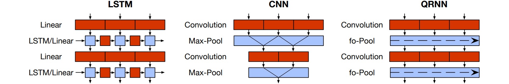
QRNN使用一维卷积处理输入序列,设置卷积核大小为$k$,则根据最近$k$时刻的输入$x_{t-k+1:t}$生成当前时刻的输入门$z_t$, 遗忘门$f_t$和输出门$o_t$。与LSTM不同,这一步不依赖于隐状态$h_{t-1}$,因此可以以矩阵方式并行地运算:
\[\begin{aligned} z_t &= \text{tanh}(W_{z}^{1}x_{t-k+1}+W_{z}^{2}x_{t-k+2}+\cdots + W_{z}^{k}x_{t}) \\ f_t &= \sigma(W_{f}^{1}x_{t-k+1}+W_{f}^{2}x_{t-k+2}+\cdots + W_{f}^{k}x_{t}) \\ o_t &= \sigma(W_{o}^{1}x_{t-k+1}+W_{o}^{2}x_{t-k+2}+\cdots + W_{o}^{k}x_{t}) \end{aligned}\]然后通过动态平均池化构造序列的输出(隐状态),这一步是循环实现的,是一个无参数函数:
\[\begin{aligned} c_t &= c_{t-1} \odot f_t + z_t \odot (1-f_t) \\ h_{t} &= o_t \odot c_t \end{aligned}\]使用torchqrnn库构造QRNN:
import torch
from torchqrnn import QRNN

seq_len, batch_size, hidden_size = 7, 20, 256
qrnn = QRNN(hidden_size, hidden_size, num_layers=2, dropout=0.4)
input = torch.randn(seq_len, batch_size, hidden_size)
output, hidden = qrnn(input)
(4) 简单循环单元 SRU
简单循环单元 (Simple Recurrent Unit, SRU)的设计思路与QRNN类似,通过把矩阵乘法放在串行循环之外,能够并行地处理输入序列,提升了运算速度。
SRU中每个时间步的门控计算只依赖于当前时间步的输入,并在输出(隐状态)中添加了跳跃连接:
\[\begin{aligned} \tilde{x}_t &= Wx_t \\ f_t &= \sigma(W_{f}x_{t}+b_f) \\ r_t &= \sigma(W_{r}x_{t}+b_r) \\ c_t &= c_{t-1} \odot f_t + \tilde{x}_t \odot (1-f_t) \\ h_{t} &= r_t \odot g(c_t) + (1-r_t) \odot x_t \end{aligned}\]
(5) 有序神经元LSTM ON-LSTM
ON-LSTM通过有序神经元(Ordered Neuron)把层级结构(树结构)整合到LSTM中,从而允许LSTM无监督地学习到层级结构信息(如句子的句法结构)。
ON-LSTM假设神经元$c_t$已经排好序,$c_t$中索引值越小的元素表示越低层级的信息,而索引值越大的元素表示越高层级的信息;并引入了主遗忘门\(\tilde{f}_t\)和主输入门\(\tilde{i}_t\),分别代表$c_{t-1}$中的历史信息层级$d_f$和\(\hat{c}_t\)中的输入信息层级$d_i$。
当前输入\(\hat{c}_t\)更容易影响低层信息,所以对神经元影响的索引范围是$[0,d_i]$;历史信息$c_{t-1}$保留的是高层信息,所以影响的范围是$[d_f,d_{\max}]$;在重叠部分$[d_f,d_i]$通过LSTM的形式更新记忆状态。
\[\begin{aligned} i_t &= \sigma(W_{i}x_t+U_{i}h_{t-1}+b_i) \\ f_t &= \sigma(W_{f}x_t+U_{f}h_{t-1}+b_f) \\ o_t &= \sigma(W_{o}x_t+U_{o}h_{t-1}+b_o) \\ \hat{c}_t &= \text{tanh}(W_{c}x_t+U_{c}h_{t-1}+b_c) \\ \tilde{f}_t &= \text{cumsum}(\text{softmax}(W_{\tilde{f}}x_t+U_{\tilde{f}}h_{t-1}+b_{\tilde{f}})) \\ \tilde{i}_t &= 1- \text{cumsum}(\text{softmax}(W_{\tilde{i}}x_t+U_{\tilde{i}}h_{t-1}+b_{\tilde{i}})) \\ w_t &= \tilde{f}_t \odot \tilde{i}_t \\ c_t &= w_t\odot (f_t \odot c_{t-1} + i_t \odot \hat{c}_t) + (\tilde{f}_t-w_t) \cdot c_{t-1} + (\tilde{i}_t-w_t) \cdot \hat{c}_t \\ h_{t} &= o_t \odot \text{tanh}(c_t) \end{aligned}\]
5. 深层RNN
深层RNN通过增加循环神经网络的深度(即堆叠循环层的数量)增强循环神经网络的特征提取能力,即增加同一时刻网络输入到输出之间的路径。
(1) 堆叠循环神经网络 Stacked RNN
堆叠循环神经网络(Stacked RNN)是将多个循环网络堆叠起来。

(2) 双向循环神经网络 Bidirectional RNN
双向循环神经网络(Bidirectional RNN)由两层循环神经网络组成,它们的输入相同,只是信息传递的方向不同。


