在图像合成任务上扩散模型超越了生成对抗网络.
本文提出了一种实现条件扩散模型的事后修改(Classifier-Guidance)方法。事后修改是指在已经训练好的无条件扩散模型的基础上引入一个可训练的分类器(Classifier),用分类器来调整生成过程以实现控制生成。这类模型的训练成本比较低,但是采样成本会高一些,而且难以控制生成图像的细节。
实现扩散模型的一般思路:
- 定义前向扩散过程:\(q\left(\mathbf{x}_t \mid \mathbf{x}_{t-1}\right)\)
- 解析地推导:\(q\left(\mathbf{x}_t \mid \mathbf{x}_{0}\right)\)
- 解析地推导:\(q\left(\mathbf{x}_{t-1} \mid \mathbf{x}_t,\mathbf{x}_{0}\right)\)
- 近似反向扩散过程:\(p_{\theta}\left(\mathbf{x}_{t-1} \mid \mathbf{x}_t\right)\)
条件扩散模型是指在采样过程\(p_{\theta}\left(\mathbf{x}_{t-1} \mid \mathbf{x}_t\right)\)中引入输入条件\(\mathbf{y}\),则采样过程变为\(p_{\theta}\left(\mathbf{x}_{t-1} \mid \mathbf{x}_t,\mathbf{y}\right)\)。为了重用训练好的模型\(p_{\theta}\left(\mathbf{x}_{t-1} \mid \mathbf{x}_t\right)\),根据贝叶斯定理:
\[\begin{aligned} p_{\theta}\left(\mathbf{x}_{t-1} \mid \mathbf{x}_t,\mathbf{y}\right) &= \frac{p_{\theta}\left(\mathbf{x}_{t-1} , \mathbf{x}_t,\mathbf{y}\right)}{p_{\theta}\left(\mathbf{x}_t,\mathbf{y}\right)} \\ &= \frac{p_{\theta}\left(\mathbf{y} \mid \mathbf{x}_{t-1} , \mathbf{x}_t\right)p_{\theta}\left(\mathbf{x}_{t-1} , \mathbf{x}_t\right)}{p_{\theta}\left(\mathbf{y}\mid \mathbf{x}_t\right)p_{\theta}\left(\mathbf{x}_t\right)} \\ &= \frac{p_{\theta}\left(\mathbf{y} \mid \mathbf{x}_{t-1} , \mathbf{x}_t\right)p_{\theta}\left(\mathbf{x}_{t-1} \mid \mathbf{x}_t\right)}{p_{\theta}\left(\mathbf{y}\mid \mathbf{x}_t\right)} \\ &= \frac{p_{\theta}\left(\mathbf{y} \mid \mathbf{x}_{t-1}\right)p_{\theta}\left(\mathbf{x}_{t-1} \mid \mathbf{x}_t\right)}{p_{\theta}\left(\mathbf{y}\mid \mathbf{x}_t\right)} \\ &= p_{\theta}\left(\mathbf{x}_{t-1} \mid \mathbf{x}_t\right) e^{\log p_{\theta}\left(\mathbf{y} \mid \mathbf{x}_{t-1}\right) - \log p_{\theta}\left(\mathbf{y} \mid \mathbf{x}_t\right)} \end{aligned}\]为了进一步得到可采样的近似结果,在\(\mathbf{x}_{t-1}=\boldsymbol{\mu}_\theta\left(\mathbf{x}_t, t\right)\)处考虑泰勒展开:
\[\begin{aligned} \log p_{\theta}\left(\mathbf{y} \mid \mathbf{x}_{t-1}\right) \approx \log p_{\theta}\left(\mathbf{y} \mid \mathbf{x}_t\right) + (\mathbf{x}_{t-1}-\boldsymbol{\mu}_\theta\left(\mathbf{x}_t, t\right)) \cdot \nabla_{\mathbf{x}_t} \log p_{\theta}\left(\mathbf{y} \mid \mathbf{x}_t\right)|_{\mathbf{x}_t=\boldsymbol{\mu}_\theta\left(\mathbf{x}_t, t\right)} + \mathcal{O}(\mathbf{x}_t) \end{aligned}\]并注意到反向扩散过程的建模:
\[\begin{aligned} p_\theta\left(\mathbf{x}_{t-1} \mid \mathbf{x}_t\right)&=\mathcal{N}\left(\mathbf{x}_{t-1} ; \boldsymbol{\mu}_\theta\left(\mathbf{x}_t, t\right), \sigma_t^2 \mathbf{I}\right) \\ \end{aligned}\]因此有:
\[\begin{aligned} p_{\theta}\left(\mathbf{x}_{t-1} \mid \mathbf{x}_t,\mathbf{y}\right) &=p_{\theta}\left(\mathbf{x}_{t-1} \mid \mathbf{x}_t\right) e^{\log p_{\theta}\left(\mathbf{y} \mid \mathbf{x}_{t-1}\right) - \log p_{\theta}\left(\mathbf{y} \mid \mathbf{x}_t\right)} \\ &\propto \exp\left(-\frac{\left\| \mathbf{x}_{t-1} -\boldsymbol{\mu}_\theta\left(\mathbf{x}_t, t\right) \right\|^2}{2\sigma_t^2}+(\mathbf{x}_{t-1}-\boldsymbol{\mu}_\theta\left(\mathbf{x}_t, t\right)) \cdot \nabla_{\mathbf{x}_t} \log p_{\theta}\left(\mathbf{y} \mid \mathbf{x}_t\right)|_{\mathbf{x}_t=\boldsymbol{\mu}_\theta\left(\mathbf{x}_t, t\right)} + \mathcal{O}(\mathbf{x}_t) \right) \\ &\propto \exp\left(-\frac{\left\| \mathbf{x}_{t-1} -\boldsymbol{\mu}_\theta\left(\mathbf{x}_t, t\right)-\sigma_t^2 \nabla_{\mathbf{x}_t} \log p_{\theta}\left(\mathbf{y} \mid \mathbf{x}_t\right)|_{\mathbf{x}_t=\boldsymbol{\mu}_\theta\left(\mathbf{x}_t, t\right)}\right\|^2}{2\sigma_t^2} + \mathcal{O}(\mathbf{x}_t) \right) \\ \end{aligned}\]则\(p_{\theta}\left(\mathbf{x}_{t-1} \mid \mathbf{x}_t,\mathbf{y}\right)\)近似服从正态分布:
\[\begin{aligned} p_{\theta}\left(\mathbf{x}_{t-1} \mid \mathbf{x}_t,\mathbf{y}\right)=\mathcal{N}\left(\mathbf{x}_{t-1} ; \boldsymbol{\mu}_\theta\left(\mathbf{x}_t, t\right)+\sigma_t^2 \nabla_{\mathbf{x}_t} \log p_{\theta}\left(\mathbf{y} \mid \mathbf{x}_t\right)|_{\mathbf{x}_t=\boldsymbol{\mu}_\theta\left(\mathbf{x}_t, t\right)}, \sigma_t^2 \mathbf{I}\right) \\ \end{aligned}\]因此条件扩散模型\(p_{\theta}\left(\mathbf{x}_{t-1} \mid \mathbf{x}_t,\mathbf{y}\right)\)的采样过程为:
\[\mathbf{x}_{t-1} = \boldsymbol{\mu}_\theta\left(\mathbf{x}_t, t\right)+\underbrace{\sigma_t^2 \nabla_{\mathbf{x}_t} \log p_{\theta}\left(\mathbf{y} \mid \mathbf{x}_t\right)|_{\mathbf{x}_t=\boldsymbol{\mu}_\theta\left(\mathbf{x}_t, t\right)}}_{\text{新增项}}+ \sigma_t \mathbf{z},\mathbf{z} \sim \mathcal{N}\left(\mathbf{0}, \mathbf{I}\right)\]向分类器的梯度中引入一个缩放参数$γ$,可以更好地调节生成效果:
\[\mathbf{x}_{t-1} = \boldsymbol{\mu}_\theta\left(\mathbf{x}_t, t\right)+\sigma_t^2 \gamma \nabla_{\mathbf{x}_t} \log p_{\theta}\left(\mathbf{y} \mid \mathbf{x}_t\right)|_{\mathbf{x}_t=\boldsymbol{\mu}_\theta\left(\mathbf{x}_t, t\right)}+ \sigma_t \mathbf{z},\mathbf{z} \sim \mathcal{N}\left(\mathbf{0}, \mathbf{I}\right)\]当$γ>1$时,生成过程将使用更多的分类器信号,结果将会提高生成结果与输入信号$y$的相关性,但是会相应地降低生成结果的多样性;反之,则会降低生成结果与输入信号之间的相关性,但增加了多样性。
缩放参数$γ$相当于通过幂操作来提高分布的聚焦程度,即定义:
\[\tilde{p}_{\theta}\left(\mathbf{y} \mid \mathbf{x}_t\right) = \frac{p_{\theta}^{\gamma}\left(\mathbf{y} \mid \mathbf{x}_t\right)}{\sum_{\mathbf{y}} p_{\theta}^{\gamma}\left(\mathbf{y} \mid \mathbf{x}_t\right)}\]随着$γ$的增大,\(\tilde{p}_{\theta}\left(\mathbf{y} \mid \mathbf{x}_t\right)\)的预测会越来越接近one hot分布,生成过程会倾向于挑出分类置信度很高的样本。
⚪ 实现条件扩散模型
实现事后修改的条件扩散模型的关键在于计算\(\nabla_{\mathbf{x}_t} \log p_{\theta}\left(\mathbf{y} \mid \mathbf{x}_t\right)\),把\(p_{\theta}\left(\mathbf{y} \mid \mathbf{x}_t\right)\)定义为一个(预训练的)分类器,则该梯度项的计算实现为:
class Classifier(nn.Module):
   def __init__(self, image_size, num_classes, t_dim=1) -> None:
      super().__init__()
      self.linear_t = nn.Linear(t_dim, num_classes)
      self.linear_img = nn.Linear(image_size * image_size * 3, num_classes)

  def forward(self, x, t):
      """
      Args:
          x (_type_): [B, 3, N, N]
          t (_type_): [B,]
      Returns:
              logits [B, num_classes]
      """
      B = x.shape[0]
      t = t.view(B, 1)
      logits = self.linear_t(t.float()) + self.linear_img(x.view(x.shape[0], -1))
      return logits

def classifier_cond_fn(x, t, classifier, y, classifier_scale=1):
  """
  return the graident of the classifier outputing y wrt x.
  formally expressed as d_log(classifier(x, t)) / dx
  """
  assert y is not None
  with torch.enable_grad():
      x_in = x.detach().requires_grad_(True)
      logits = classifier(x_in, t)
      log_probs = F.log_softmax(logits, dim=-1)
      selected = log_probs[range(len(logits)), y.view(-1)]
      grad = torch.autograd.grad(selected.sum(), x_in)[0] * classifier_scale
      return grad
对于DDPM,实现条件采样只需在采样时增加估计均值的修正项:
\[\mathbf{x}_{t-1} = \boldsymbol{\mu}_\theta\left(\mathbf{x}_t, t\right)+\underbrace{\sigma_t^2 \nabla_{\mathbf{x}_t} \log p_{\theta}\left(\mathbf{y} \mid \mathbf{x}_t\right)|_{\mathbf{x}_t=\boldsymbol{\mu}_\theta\left(\mathbf{x}_t, t\right)}}_{\text{新增项}}+ \sigma_t \mathbf{z},\mathbf{z} \sim \mathcal{N}\left(\mathbf{0}, \mathbf{I}\right)\]
def condition_mean(self, mean,variance, x, t, guidance_kwargs=None):
  """
  Compute the mean for the previous step, given a function cond_fn that
  computes the gradient of a conditional log probability with respect to
  x. In particular, cond_fn computes grad(log(p(y|x))), and we want to
  condition on y.
  """
  gradient = self.classifier_cond_fn(x, t, **guidance_kwargs)
  new_mean = (
      mean.float() + variance * gradient.float()
  )
  # print("gradient: ",(variance * gradient.float()).mean())
  return new_mean
对于DDIM,实现条件采样只需在采样时增加估计噪声的修正项:
\[\begin{aligned} \tilde{\boldsymbol{\epsilon}}_\theta\left(\mathbf{x}_t, t\right) = \boldsymbol{\epsilon}_\theta\left(\mathbf{x}_t, t\right)-\sqrt{1-\bar{\alpha}_t}\nabla_{\mathbf{x}} \log p_t(\mathbf{y}\mid \mathbf{x}) \end{aligned}\]对应的采样过程为:
\[\begin{aligned} \mathbf{x}_{t-1} = \frac{1}{\sqrt{\alpha_t}}\mathbf{x}_{t}+\left( \sqrt{1-\bar{\alpha}_{t-1}-\sigma_t^2}-\frac{\sqrt{1-\bar{\alpha}_t}}{\sqrt{\alpha_t}} \right) \tilde{\boldsymbol{\epsilon}}_\theta\left(\mathbf{x}_t, t\right)+ \sigma_t \mathbf{z} \end{aligned}\]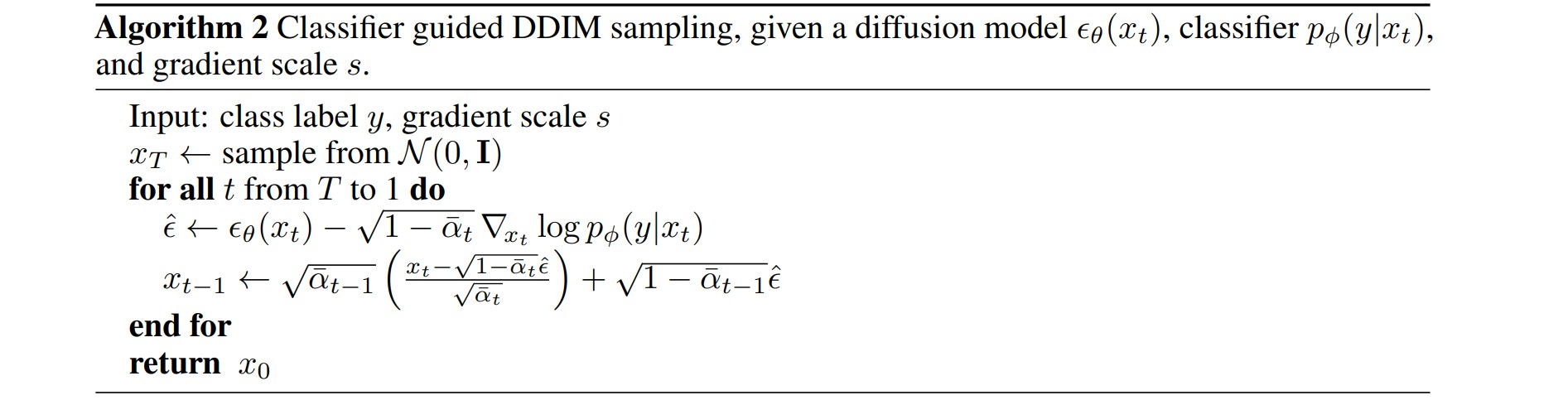
@torch.no_grad()
def ddim_sample(self, shape, return_all_timesteps = False, guidance_kwargs=None):
  batch, device, total_timesteps, sampling_timesteps, eta = shape[0], self.betas.device, self.num_timesteps, self.sampling_timesteps, self.ddim_sampling_eta

  times = torch.linspace(-1, total_timesteps - 1, steps = sampling_timesteps + 1)   # [-1, 0, 1, 2, ..., T-1] when sampling_timesteps == total_timesteps
  times = list(reversed(times.int().tolist()))
  time_pairs = list(zip(times[:-1], times[1:])) # [(T-1, T-2), (T-2, T-3), ..., (1, 0), (0, -1)]

  img = torch.randn(shape, device = device)
  imgs = [img]

  x_start = None

  for time, time_next in tqdm(time_pairs, desc = 'sampling loop time step'):
      time_cond = torch.full((batch,), time, device = device, dtype = torch.long)
      pred_noise = self.model(img, time_cond) # 计算 \epsilon(x_t, t)
      x_start = self.predict_start_from_noise(img, time_cond, pred_noise) # x_0

      if time_next < 0:
          img = x_start
          imgs.append(img)
          continue

      alpha = self.alphas_cumprod[time]
      alpha_next = self.alphas_cumprod[time_next]
      beta = self.betas_cumprod[time]

      sigma = eta * ((1 - alpha / alpha_next) * (1 - alpha_next) / (1 - alpha)).sqrt()
      c = (1 - alpha_next - sigma ** 2).sqrt()

      if exists(guidance_kwargs):
          gradient = self.classifier_cond_fn(img, time, **guidance_kwargs)

      noise = torch.randn_like(img)
      img = x_start * alpha_next.sqrt() + \
            c * pred_noise + \
            sigma * noise

      if exists(guidance_kwargs):
          img = img + ((beta * (1 - alpha) / (alpha / alpha_next)).sqrt() - beta.sqrt() * c)* gradient.float()

      imgs.append(img)

  ret = img if not return_all_timesteps else torch.stack(imgs, dim = 1)
  ret = (ret + 1) * 0.5
  return ret
基于事后修改的条件扩散模型的完整实现可参考denoising-diffusion-pytorch。


