DDPM:去噪扩散概率模型.
1. 扩散模型
扩散模型 (Diffusion Model)是一类受到非平衡热力学 (non-equilibrium thermodynamics)启发的深度生成模型。这类模型首先定义前向扩散过程的马尔科夫链 (Markov Chain),向数据中逐渐地添加随机噪声;然后学习反向扩散过程,从噪声中构造所需的数据样本。扩散模型也是一类隐变量模型,其隐变量通常具有较高的维度(与原始数据相同的维度)。

(1)前向扩散过程 forward diffusion process
给定从真实数据分布$q(\mathbf{x})$中采样的数据点$\mathbf{x}_0$~$q(\mathbf{x})$,前向扩散过程定义为逐渐向样本中添加高斯噪声(共计$T$步),从而产生一系列噪声样本$\mathbf{x}_1,…,\mathbf{x}_T$。噪声的添加程度是由一系列方差系数\(\{\beta_t\in (0,1)\}_{t=1}^T\)控制的。
\[\begin{aligned} q\left(\mathbf{x}_t \mid \mathbf{x}_{t-1}\right)&=\mathcal{N}\left(\mathbf{x}_t ; \sqrt{1-\beta_t} \mathbf{x}_{t-1}, \beta_t \mathbf{I}\right) \\ q\left(\mathbf{x}_{1: T} \mid \mathbf{x}_0\right)&=\prod_{t=1}^T q\left(\mathbf{x}_t \mid \mathbf{x}_{t-1}\right) \end{aligned}\]在前向扩散过程中,数据样本$\mathbf{x}_0$逐渐丢失其具有判别性的特征;当$T \to \infty$时,$\mathbf{x}_T$等价于一个各向同性的高斯分布。
使用重参数化技巧,可以采样任意时刻$t$对应的噪声样本$\mathbf{x}_t$。若记$\alpha_t = 1- \beta_t$,则有:
\[\begin{array}{rlr} \mathbf{x}_t & =\sqrt{\alpha_t} \mathbf{x}_{t-1}+\sqrt{1-\alpha_t} \boldsymbol{\epsilon}_{t-1} \quad ; \text { where } \boldsymbol{\epsilon}_{t-1}, \boldsymbol{\epsilon}_{t-2}, \cdots \sim \mathcal{N}(\mathbf{0}, \mathbf{I}) \\ & =\sqrt{\alpha_t \alpha_{t-1}} \mathbf{x}_{t-2}+\sqrt{\alpha_t(1-\alpha_{t-1})} \boldsymbol{\epsilon}_{t-2}+\sqrt{1-\alpha_t} \boldsymbol{\epsilon}_{t-1} \\ & \left( \text { Note that } \mathcal{N}(\mathbf{0}, \alpha_t(1-\alpha_{t-1})) + \mathcal{N}(\mathbf{0}, 1-\alpha_{t}) = \mathcal{N}(\mathbf{0}, 1-\alpha_t\alpha_{t-1}) \right)\\ & =\sqrt{\alpha_t \alpha_{t-1}} \mathbf{x}_{t-2}+\sqrt{1-\alpha_t \alpha_{t-1}} \overline{\boldsymbol{\epsilon}}_{t-2} \\ & =\cdots \\ & =\sqrt{\prod_{i=1}^t \alpha_i} \mathbf{x}_0+\sqrt{1-\prod_{i=1}^t \alpha_i} \boldsymbol{\epsilon} \\ & =\sqrt{\bar{\alpha}_t} \mathbf{x}_0+\sqrt{1-\bar{\alpha}_t} \boldsymbol{\epsilon} \\ q\left(\mathbf{x}_t \mid \mathbf{x}_0\right) & =\mathcal{N}\left(\mathbf{x}_t ; \sqrt{\bar{\alpha}_t} \mathbf{x}_0,\left(1-\bar{\alpha}_t\right) \mathbf{I}\right) & \end{array}\]通常在前向扩散过程中会逐渐增大添加噪声的程度,即$\beta_1<\beta_2<\cdots < \beta_T$;因此有$\bar{\alpha}_1>\cdots>\bar{\alpha}_T$。
(2)反向扩散过程 reverse diffusion process
如果能够求得前向扩散过程\(q\left(\mathbf{x}_t \mid \mathbf{x}_{t-1}\right)\)的逆过程\(q\left(\mathbf{x}_{t-1} \mid \mathbf{x}_{t}\right)\),则能够从高斯噪声输入\(\mathbf{x}_T \sim \mathcal{N}(\mathbf{0}, \mathbf{I})\)中构造真实样本。注意到当$\beta_t$足够小时,\(q\left(\mathbf{x}_{t-1} \mid \mathbf{x}_{t}\right)\)也近似服从高斯分布。然而直接估计\(q\left(\mathbf{x}_{t-1} \mid \mathbf{x}_{t}\right)\)是相当困难的,我们在给定数据集的基础上通过神经网络学习条件概率\(p_{\theta}\left(\mathbf{x}_{t-1} \mid \mathbf{x}_{t}\right)\):
\[\begin{aligned} p_\theta\left(\mathbf{x}_{0: T}\right)&=p\left(\mathbf{x}_T\right) \prod_{t=1}^T p_\theta\left(\mathbf{x}_{t-1} \mid \mathbf{x}_t\right) \\ p_\theta\left(\mathbf{x}_{t-1} \mid \mathbf{x}_t\right)&=\mathcal{N}\left(\mathbf{x}_{t-1} ; \boldsymbol{\mu}_\theta\left(\mathbf{x}_t, t\right), \boldsymbol{\Sigma}_\theta\left(\mathbf{x}_t, t\right)\right) \end{aligned}\]注意到如果额外引入条件\(\mathbf{x}_0\),则\(q\left(\mathbf{x}_{t-1} \mid \mathbf{x}_{t},\mathbf{x}_0\right)\)是可解的:
\[\begin{aligned} q\left(\mathbf{x}_{t-1} \mid \mathbf{x}_t, \mathbf{x}_0\right) & =q\left(\mathbf{x}_t \mid \mathbf{x}_{t-1}, \mathbf{x}_0\right) \frac{q\left(\mathbf{x}_{t-1} \mid \mathbf{x}_0\right)}{q\left(\mathbf{x}_t \mid \mathbf{x}_0\right)} \\ & \propto \exp \left(-\frac{1}{2}\left(\frac{\left(\mathbf{x}_t-\sqrt{\alpha_t} \mathbf{x}_{t-1}\right)^2}{\beta_t}+\frac{\left(\mathbf{x}_{t-1}-\sqrt{\bar{\alpha}_{t-1}} \mathbf{x}_0\right)^2}{1-\bar{\alpha}_{t-1}}-\frac{\left(\mathbf{x}_t-\sqrt{\bar{\alpha}_t} \mathbf{x}_0\right)^2}{1-\bar{\alpha}_t}\right)\right) \\ & =\exp \left(-\frac{1}{2}\left(\frac{\mathbf{x}_t^2-2 \sqrt{\alpha_t} \mathbf{x}_t \mathbf{x}_{t-1}+\alpha_t \mathbf{x}_{t-1}^2}{\beta_t}+\frac{\mathbf{x}_{t-1}^2-2 \sqrt{\bar{\alpha}_{t-1}} \mathbf{x}_0 \mathbf{x}_{t-1}+\bar{\alpha}_{t-1} \mathbf{x}_0^2}{1-\bar{\alpha}_{t-1}}-\frac{\left(\mathbf{x}_t-\sqrt{\bar{\alpha}_t} \mathbf{x}_0\right)^2}{1-\bar{\alpha}_t}\right)\right) \\ & =\exp \left(-\frac{1}{2}\left(\left(\frac{\alpha_t}{\beta_t}+\frac{1}{1-\bar{\alpha}_{t-1}}\right) \mathbf{x}_{t-1}^2-\left(\frac{2 \sqrt{\alpha_t}}{\beta_t} \mathbf{x}_t+\frac{2 \sqrt{\bar{\alpha}_{t-1}}}{1-\bar{\alpha}_{t-1}} \mathbf{x}_0\right) \mathbf{x}_{t-1}+C\left(\mathbf{x}_t, \mathbf{x}_0\right)\right)\right) \end{aligned}\]其中\(C\left(\mathbf{x}_t, \mathbf{x}_0\right)\)是与\(\mathbf{x}_{t-1}\)无关的项。因此\(q\left(\mathbf{x}_{t-1} \mid \mathbf{x}_{t},\mathbf{x}_0\right)\)也服从高斯分布:
\[\begin{aligned} q\left(\mathbf{x}_{t-1} \mid \mathbf{x}_t, \mathbf{x}_0\right) & =\mathcal{N}\left(\mathbf{x}_{t-1} ; \tilde{\boldsymbol{\mu}}\left(\mathbf{x}_t, \mathbf{x}_0\right), \tilde{\beta}_t \mathbf{I}\right) \\ \tilde{\beta}_t & =1 /\left(\frac{\alpha_t}{\beta_t}+\frac{1}{1-\bar{\alpha}_{t-1}}\right)=1 /\left(\frac{\alpha_t-\bar{\alpha}_t+\beta_t}{\beta_t\left(1-\bar{\alpha}_{t-1}\right)}\right)=\frac{1-\bar{\alpha}_{t-1}}{1-\bar{\alpha}_t} \cdot \beta_t \\ \tilde{\boldsymbol{\mu}}_t\left(\mathbf{x}_t, \mathbf{x}_0\right) & =\left(\frac{\sqrt{\alpha_t}}{\beta_t} \mathbf{x}_t+\frac{\sqrt{\bar{\alpha}_{t-1}}}{1-\bar{\alpha}_{t-1}} \mathbf{x}_0\right) /\left(\frac{\alpha_t}{\beta_t}+\frac{1}{1-\bar{\alpha}_{t-1}}\right) \\ & =\left(\frac{\sqrt{\alpha_t}}{\beta_t} \mathbf{x}_t+\frac{\sqrt{\bar{\alpha}_{t-1}}}{1-\bar{\alpha}_{t-1}} \mathbf{x}_0\right) \frac{1-\bar{\alpha}_{t-1}}{1-\bar{\alpha}_t} \cdot \beta_t \\ & =\frac{\sqrt{\alpha_t}\left(1-\bar{\alpha}_{t-1}\right)}{1-\bar{\alpha}_t} \mathbf{x}_t+\frac{\sqrt{\bar{\alpha}_{t-1}} \beta_t}{1-\bar{\alpha}_t} \mathbf{x}_0 \end{aligned}\]注意到$\mathbf{x}_t=\sqrt{\bar{\alpha}_t} \mathbf{x}_0+\sqrt{1-\bar{\alpha}_t} \boldsymbol{\epsilon}$,因此把$\mathbf{x}_0=(\mathbf{x}_t-\sqrt{1-\bar{\alpha}_t} \boldsymbol{\epsilon})/\sqrt{\bar{\alpha}_t}$代入$\tilde{\boldsymbol{\mu}}_t$可得:
\[\begin{aligned} \tilde{\boldsymbol{\mu}}_t & =\frac{\sqrt{\alpha_t}\left(1-\bar{\alpha}_{t-1}\right)}{1-\bar{\alpha}_t} \mathbf{x}_t+\frac{\sqrt{\bar{\alpha}_{t-1}} \beta_t}{1-\bar{\alpha}_t} \frac{1}{\sqrt{\bar{\alpha}_t}}\left(\mathbf{x}_t-\sqrt{1-\bar{\alpha}_t} \boldsymbol{\epsilon}_t\right) \\ & =\frac{1}{\sqrt{\alpha_t}}\left(\mathbf{x}_t-\frac{1-\alpha_t}{\sqrt{1-\bar{\alpha}_t}} \epsilon_t\right) \end{aligned}\](3)目标函数
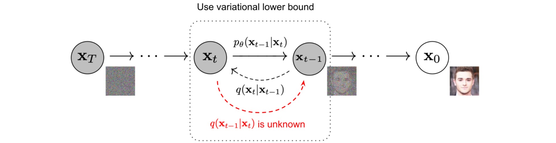
扩散模型的目标函数为最小化\(p_\theta\left(\mathbf{x}_{0}\right)\)的负对数似然\(\log p_\theta\left(\mathbf{x}_0\right)\):
\[\begin{aligned} -\log p_\theta\left(\mathbf{x}_0\right) & \leq-\log p_\theta\left(\mathbf{x}_0\right)+D_{\mathrm{KL}}\left(q\left(\mathbf{x}_{1: T} \mid \mathbf{x}_0\right) \| p_\theta\left(\mathbf{x}_{1: T} \mid \mathbf{x}_0\right)\right) \\ & =-\log p_\theta\left(\mathbf{x}_0\right)+\mathbb{E}_{\mathbf{x}_{1: T} \sim q\left(\mathbf{x}_{\left.1: T\right.} \mid \mathbf{x}_0\right)}\left[\log \frac{q\left(\mathbf{x}_{1: T} \mid \mathbf{x}_0\right)}{p_\theta\left(\mathbf{x}_{0: T}\right) / p_\theta\left(\mathbf{x}_0\right)}\right] \\ & =-\log p_\theta\left(\mathbf{x}_0\right)+\mathbb{E}_q\left[\log \frac{q\left(\mathbf{x}_{1: T} \mid \mathbf{x}_0\right)}{p_\theta\left(\mathbf{x}_{0: T}\right)}+\log p_\theta\left(\mathbf{x}_0\right)\right] \\ & =\mathbb{E}_q\left[\log \frac{q\left(\mathbf{x}_{1: T} \mid \mathbf{x}_0\right)}{p_\theta\left(\mathbf{x}_{0: T}\right)}\right] \\ \end{aligned}\]可以构造负对数似然的负变分下界 (variational lower bound):
\[L_{\mathrm{VLB}}=\mathbb{E}_{q\left(\mathbf{x}_{0: T}\right)}\left[\log \frac{q\left(\mathbf{x}_{1: T} \mid \mathbf{x}_0\right)}{p_\theta\left(\mathbf{x}_{0: T}\right)}\right] \geq-\mathbb{E}_{q\left(\mathbf{x}_0\right)} \log p_\theta\left(\mathbf{x}_0\right)\]为了把变分下界公式中的每个项转换为可计算的,可以将上述目标进一步重写为几个KL散度项和熵项的组合:
\[\begin{aligned} & L_{\mathrm{VLB}}=\mathbb{E}_{q\left(\mathbf{x}_{0: T}\right)}\left[\log \frac{q\left(\mathbf{x}_{1: T} \mid \mathbf{x}_0\right)}{p_\theta\left(\mathbf{x}_{0: T}\right)}\right] \\ & =\mathbb{E}_q\left[\log \frac{\prod_{t=1}^T q\left(\mathbf{x}_t \mid \mathbf{x}_{t-1}\right)}{p_\theta\left(\mathbf{x}_T\right) \prod_{t=1}^T p_\theta\left(\mathbf{x}_{t-1} \mid \mathbf{x}_t\right)}\right] \\ & =\mathbb{E}_q\left[-\log p_\theta\left(\mathbf{x}_T\right)+\sum_{t=1}^T \log \frac{q\left(\mathbf{x}_t \mid \mathbf{x}_{t-1}\right)}{p_\theta\left(\mathbf{x}_{t-1} \mid \mathbf{x}_t\right)}\right] \\ & =\mathbb{E}_q\left[-\log p_\theta\left(\mathbf{x}_T\right)+\sum_{t=2}^T \log \frac{q\left(\mathbf{x}_t \mid \mathbf{x}_{t-1}\right)}{p_\theta\left(\mathbf{x}_{t-1} \mid \mathbf{x}_t\right)}+\log \frac{q\left(\mathbf{x}_1 \mid \mathbf{x}_0\right)}{p_\theta\left(\mathbf{x}_0 \mid \mathbf{x}_1\right)}\right] \\ & =\mathbb{E}_q\left[-\log p_\theta\left(\mathbf{x}_T\right)+\sum_{t=2}^T \log \left(\frac{q\left(\mathbf{x}_{t-1} \mid \mathbf{x}_t, \mathbf{x}_0\right)}{p_\theta\left(\mathbf{x}_{t-1} \mid \mathbf{x}_t\right)} \cdot \frac{q\left(\mathbf{x}_t \mid \mathbf{x}_0\right)}{q\left(\mathbf{x}_{t-1} \mid \mathbf{x}_0\right)}\right)+\log \frac{q\left(\mathbf{x}_1 \mid \mathbf{x}_0\right)}{p_\theta\left(\mathbf{x}_0 \mid \mathbf{x}_1\right)}\right] \\ & =\mathbb{E}_q\left[-\log p_\theta\left(\mathbf{x}_T\right)+\sum_{t=2}^T \log \frac{q\left(\mathbf{x}_{t-1} \mid \mathbf{x}_t, \mathbf{x}_0\right)}{p_\theta\left(\mathbf{x}_{t-1} \mid \mathbf{x}_t\right)}+\sum_{t=2}^T \log \frac{q\left(\mathbf{x}_t \mid \mathbf{x}_0\right)}{q\left(\mathbf{x}_{t-1} \mid \mathbf{x}_0\right)}+\log \frac{q\left(\mathbf{x}_1 \mid \mathbf{x}_0\right)}{p_\theta\left(\mathbf{x}_0 \mid \mathbf{x}_1\right)}\right] \\ & =\mathbb{E}_q\left[-\log p_\theta\left(\mathbf{x}_T\right)+\sum_{t=2}^T \log \frac{q\left(\mathbf{x}_{t-1} \mid \mathbf{x}_t, \mathbf{x}_0\right)}{p_\theta\left(\mathbf{x}_{t-1} \mid \mathbf{x}_t\right)}+\log \frac{q\left(\mathbf{x}_T \mid \mathbf{x}_0\right)}{q\left(\mathbf{x}_1 \mid \mathbf{x}_0\right)}+\log \frac{q\left(\mathbf{x}_1 \mid \mathbf{x}_0\right)}{p_\theta\left(\mathbf{x}_0 \mid \mathbf{x}_1\right)}\right] \\ & =\mathbb{E}_q\left[\log \frac{q\left(\mathbf{x}_T \mid \mathbf{x}_0\right)}{p_\theta\left(\mathbf{x}_T\right)}+\sum_{t=2}^T \log \frac{q\left(\mathbf{x}_{t-1} \mid \mathbf{x}_t, \mathbf{x}_0\right)}{p_\theta\left(\mathbf{x}_{t-1} \mid \mathbf{x}_t\right)}-\log p_\theta\left(\mathbf{x}_0 \mid \mathbf{x}_1\right)\right] \\ & =\mathbb{E}_q[\underbrace{D_{\mathrm{KL}}\left(q\left(\mathbf{x}_T \mid \mathbf{x}_0\right) \| p_\theta\left(\mathbf{x}_T\right)\right)}_{L_T}+\sum_{t=2}^T \underbrace{D_{\mathrm{KL}}\left(q\left(\mathbf{x}_{t-1} \mid \mathbf{x}_t, \mathbf{x}_0\right) \| p_\theta\left(\mathbf{x}_{t-1} \mid \mathbf{x}_t\right)\right)}_{L_{t-1}}-\underbrace{\log p_\theta\left(\mathbf{x}_0 \mid \mathbf{x}_1\right)}_{L_0}] \\ \end{aligned}\]至此,扩散模型的目标函数(负变分下界)可以被分解为$T$项:
\[\begin{aligned} L_{\mathrm{VLB}} & =L_T+L_{T-1}+\cdots+L_0 \\ \text { where } L_T & =D_{\mathrm{KL}}\left(q\left(\mathbf{x}_T \mid \mathbf{x}_0\right) \| p_\theta\left(\mathbf{x}_T\right)\right) \\ L_t & =D_{\mathrm{KL}}\left(q\left(\mathbf{x}_t \mid \mathbf{x}_{t+1}, \mathbf{x}_0\right) \| p_\theta\left(\mathbf{x}_t \mid \mathbf{x}_{t+1}\right)\right) \text { for } 1 \leq t \leq T-1 \\ L_0 & =-\log p_\theta\left(\mathbf{x}_0 \mid \mathbf{x}_1\right) \end{aligned}\]其中$L_T$是一个常数($q$不包含可学习参数$\theta$, $\mathbf{x}_T$是高斯噪声),在训练时可以被省略;$L_0$可以通过一个离散解码器建模;而$L_t$计算了两个高斯分布的KL散度,可以得到闭式解。根据之前的讨论,我们有:
\[\begin{aligned} p_\theta\left(\mathbf{x}_{t-1} \mid \mathbf{x}_t\right)&=\mathcal{N}\left(\mathbf{x}_{t-1} ; \boldsymbol{\mu}_\theta\left(\mathbf{x}_t, t\right), \boldsymbol{\Sigma}_\theta\left(\mathbf{x}_t, t\right)\right)\\ q\left(\mathbf{x}_{t-1} \mid \mathbf{x}_t, \mathbf{x}_0\right) & =\mathcal{N}\left(\mathbf{x}_{t-1} ; \frac{1}{\sqrt{\alpha_t}}\left(\mathbf{x}_t-\frac{1-\alpha_t}{\sqrt{1-\bar{\alpha}_t}} \epsilon_t\right), \frac{1-\bar{\alpha}_{t-1}}{1-\bar{\alpha}_t} \cdot \beta_t \mathbf{I}\right) \end{aligned}\]不妨把\(\boldsymbol{\mu}_\theta\left(\mathbf{x}_t, t\right)\)表示为\(\boldsymbol{\epsilon}_\theta\left(\mathbf{x}_t, t\right)\)的函数:
\[\boldsymbol{\mu}_\theta\left(\mathbf{x}_t, t\right) = \frac{1}{\sqrt{\alpha_t}}\left(\mathbf{x}_t-\frac{1-\alpha_t}{\sqrt{1-\bar{\alpha}_t}} \boldsymbol{\epsilon}_\theta\left(\mathbf{x}_t, t\right)\right)\]则损失$L_t$可以被表示为\(\boldsymbol{\epsilon}_\theta\left(\mathbf{x}_t, t\right)\)和\(\boldsymbol{\Sigma}_\theta\left(\mathbf{x}_t, t\right)\)的函数:
\[\begin{aligned} L_t & =\mathbb{E}_{\mathbf{x}_0, \boldsymbol{\epsilon}}\left[\frac{1}{2\left\|\boldsymbol{\Sigma}_\theta\left(\mathbf{x}_t, t\right)\right\|_2^2}\left\|\tilde{\boldsymbol{\mu}}_t\left(\mathbf{x}_t, \mathbf{x}_0\right)-\boldsymbol{\mu}_\theta\left(\mathbf{x}_t, t\right)\right\|^2\right] \\ & =\mathbb{E}_{\mathbf{x}_0, \boldsymbol{\epsilon}}\left[\frac{1}{2\left\|\boldsymbol{\Sigma}_\theta\right\|_2^2}\left\|\frac{1}{\sqrt{\alpha_t}}\left(\mathbf{x}_t-\frac{1-\alpha_t}{\sqrt{1-\bar{\alpha}_t}} \boldsymbol{\epsilon}_t\right)-\frac{1}{\sqrt{\alpha_t}}\left(\mathbf{x}_t-\frac{1-\alpha_t}{\sqrt{1-\bar{\alpha}_t}} \boldsymbol{\epsilon}_\theta\left(\mathbf{x}_t, t\right)\right)\right\|^2\right] \\ & =\mathbb{E}_{\mathbf{x}_0, \boldsymbol{\epsilon}}\left[\frac{\left(1-\alpha_t\right)^2}{2 \alpha_t\left(1-\bar{\alpha}_t\right)\left\|\boldsymbol{\Sigma}_\theta\right\|_2^2}\left\|\boldsymbol{\epsilon}_t-\boldsymbol{\epsilon}_\theta\left(\mathbf{x}_t, t\right)\right\|^2\right] \\ & =\mathbb{E}_{\mathbf{x}_0, \boldsymbol{\epsilon}}\left[\frac{\left(1-\alpha_t\right)^2}{2 \alpha_t\left(1-\bar{\alpha}_t\right)\left\|\boldsymbol{\Sigma}_\theta\right\|_2^2}\left\|\boldsymbol{\epsilon}_t-\boldsymbol{\epsilon}_\theta\left(\sqrt{\bar{\alpha}_t} \mathbf{x}_0+\sqrt{1-\bar{\alpha}_t} \boldsymbol{\epsilon}_t, t\right)\right\|^2\right] \end{aligned}\]2. 一些化简
(1)参数化 $L_0$
\[\begin{aligned} L_0 & =-\log p_\theta\left(\mathbf{x}_0 \mid \mathbf{x}_1\right) \end{aligned}\]使用一个离散解码器单独参数化$L_0$:
\[\begin{aligned} p_\theta\left(\mathbf{x}_{0} \mid \mathbf{x}_1\right)&=\mathcal{N}\left(\mathbf{x}_{0} ; \boldsymbol{\mu}_\theta\left(\mathbf{x}_1, 1\right), \boldsymbol{\Sigma}_\theta\left(\mathbf{x}_1, 1\right)\right) \end{aligned}\](2)参数化 $\beta_{t}$
前向方差$\beta_1,…,\beta_T$被设置为一系列线性增加的常数,其中$\beta_1=10^{-4},\beta_T=0.02$。相对于归一化为$[-1,1]$的图像像素值,$\beta_t$通常是比较小的。扩散模型在实验中显示了高质量的生成样本,但仍然不能像其他生成模型那样取得较大的模型对数似然。
def linear_beta_schedule(timesteps=1000):
    scale = 1000 / timesteps
    beta_start = scale * 0.0001
    beta_end = scale * 0.02
    return torch.linspace(beta_start, beta_end, timesteps, dtype = torch.float64)
(3)参数化 $\Sigma_{\theta}$
可以设置$\Sigma_{\theta}(x_t,t)=\sigma_t^2\mathbf{I}$,其中$\sigma_t^2=\beta_t$或者\(\sigma_t^2=\tilde{\beta}_t=\frac{1-\overline{\alpha}_{t-1}}{1-\overline{\alpha}_{t}}\cdot \beta_t\)。如果把\(\Sigma_{\theta}\)设置为可学习参数,则容易导致训练的不稳定和较差的采样质量。
betas = linear_beta_schedule(timesteps)

alphas = 1. - betas
alphas_cumprod = torch.cumprod(alphas, dim=0)
alphas_cumprod_prev = F.pad(alphas_cumprod[:-1], (1, 0), value = 1.)
posterior_variance = betas * (1. - alphas_cumprod_prev) / (1. - alphas_cumprod)
(4)简化 $L_t$
\[\begin{aligned} L_t & =\mathbb{E}_{\mathbf{x}_0, \boldsymbol{\epsilon}}\left[\frac{\left(1-\alpha_t\right)^2}{2 \alpha_t\left(1-\bar{\alpha}_t\right)\left\|\boldsymbol{\Sigma}_\theta\right\|_2^2}\left\|\boldsymbol{\epsilon}_t-\boldsymbol{\epsilon}_\theta\left(\sqrt{\bar{\alpha}_t} \mathbf{x}_0+\sqrt{1-\bar{\alpha}_t} \boldsymbol{\epsilon}_t, t\right)\right\|^2\right] \end{aligned}\]实验表明,简化损失函数中的加权项有助于提交表现:
\[\begin{aligned} L_t^{\text {simple }} & =\mathbb{E}_{t \sim[1, T], \mathbf{x}_0, \epsilon_t}\left[\left\|\boldsymbol{\epsilon}_t-\boldsymbol{\epsilon}_\theta\left(\mathbf{x}_t, t\right)\right\|^2\right] \\ & =\mathbb{E}_{t \sim[1, T], \mathbf{x}_0, \epsilon_t}\left[\left\|\boldsymbol{\epsilon}_t-\boldsymbol{\epsilon}_\theta\left(\sqrt{\bar{\alpha}_t} \mathbf{x}_0+\sqrt{1-\bar{\alpha}_t} \boldsymbol{\epsilon}_t, t\right)\right\|^2\right] \end{aligned}\]最终目标函数为上式与一个常数之和:
\[\begin{aligned} L_{\text {simple }} & =L_t^{\text {simple }} + C \end{aligned}\]3. 实现DDPM
DDPM的训练和采样过程如下:

DDPM的实现如下。
# 按照索引t从a中取数据
def extract(a, t, x_shape):
    b, *_ = t.shape
    out = a.gather(dim=-1, index=t)
    return out.reshape(b, *((1,) * (len(x_shape) - 1)))

class GaussianDiffusion(nn.Module):
    def __init__(
        self,
        model,
        *,
        image_size,
        timesteps = 1000
    ):
        super().__init__()
        self.model = model # 用于拟合\epsilon(x_t,t)的神经网络
        self.channels = self.model.channels
        self.image_size = image_size

        betas = linear_beta_schedule(timesteps) # \beta_t
        alphas = 1. - betas # \alpha_t
        alphas_cumprod = torch.cumprod(alphas, dim=0) # \bar{\alpha}_t
        alphas_cumprod_prev = F.pad(alphas_cumprod[:-1], (1, 0), value = 1.) # \bar{\alpha}_{t-1}

        self.num_timesteps = int(timesteps)

        # helper function to register buffer from float64 to float32
        register_buffer = lambda name, val: self.register_buffer(name, val.to(torch.float32))
        register_buffer('betas', betas)

        # calculations for diffusion q(x_t | x_{t-1}) and others
        register_buffer('sqrt_alphas_cumprod', torch.sqrt(alphas_cumprod)) # \sqrt{\bar{\alpha}_t}
        register_buffer('sqrt_one_minus_alphas_cumprod', torch.sqrt(1. - alphas_cumprod)) # \sqrt{1-\bar{\alpha}_t}
        register_buffer('log_one_minus_alphas_cumprod', torch.log(1. - alphas_cumprod)) # \log{1-\bar{\alpha}_t}
        register_buffer('sqrt_recip_alphas_cumprod', torch.sqrt(1. / alphas_cumprod)) # \sqrt{1/\bar{\alpha}_t}
        register_buffer('sqrt_recipm1_alphas_cumprod', torch.sqrt(1. / alphas_cumprod - 1)) # \sqrt{1/(\bar{\alpha}_t-1)}

        # calculations for posterior q(x_{t-1} | x_t, x_0)
        posterior_variance = betas * (1. - alphas_cumprod_prev) / (1. - alphas_cumprod) # \sigma_t^2
        register_buffer('posterior_variance', posterior_variance)
        # log calculation clipped because the posterior variance is 0 at the beginning of the diffusion chain
        register_buffer('posterior_log_variance_clipped', torch.log(posterior_variance.clamp(min =1e-20)))
        register_buffer('posterior_mean_coef1', betas * torch.sqrt(alphas_cumprod_prev) / (1. - alphas_cumprod))
        register_buffer('posterior_mean_coef2', (1. - alphas_cumprod_prev) * torch.sqrt(alphas) / (1. - alphas_cumprod))

    """
    Training
    """

    # 计算x_t=\sqrt{\bat{\alpha}_t}x_0+\sqrt{1-\bat{\alpha}_t}\epsilon
    def q_sample(self, x_start, t, noise=None):
        return (
            extract(self.sqrt_alphas_cumprod, t, x_start.shape) * x_start +
            extract(self.sqrt_one_minus_alphas_cumprod, t, x_start.shape) * noise
        )

    # 计算损失函数L_t=||\epsilon-\epsilon(x_t, t)||_1
    def p_losses(self, x_start, t, noise = None):
        b, c, h, w = x_start.shape
        noise = torch.randn_like(x_start)
        target = noise

        # 计算 x_t
        x = self.q_sample(x_start = x_start, t = t, noise = noise)

        # 计算 \epsilon(x_t, t)
        model_out = self.model(x, t)

        loss = F.l1_loss(model_out, target, reduction = 'none')
        loss = reduce(loss, 'b ... -> b (...)', 'mean')
        return loss.mean()

    # 训练过程
    def forward(self, img, *args, **kwargs):
        b, c, h, w, device = *img.shape, img.device
        t = torch.randint(0, self.num_timesteps, (b,), device=device).long()

        img = img * 2 - 1 # data [0, 1] -> [-1, 1]
        return self.p_losses(img, t, *args, **kwargs)

    """
    Sampling
    """

    # 计算 x_0 = \sqrt{1/\bat{\alpha}_t}x_t-\sqrt{1/(1-\bat{\alpha}_t)}\epsilon_t
    def predict_start_from_noise(self, x_t, t, noise):
        return (
            extract(self.sqrt_recip_alphas_cumprod, t, x_t.shape) * x_t -
            extract(self.sqrt_recipm1_alphas_cumprod, t, x_t.shape) * noise
        )

    # 计算 \mu_t(x_t, x_0) = coef_1*x_0 + coef_2*x_t
    def q_posterior(self, x_start, x_t, t):
        posterior_mean = (
            extract(self.posterior_mean_coef1, t, x_t.shape) * x_start +
            extract(self.posterior_mean_coef2, t, x_t.shape) * x_t
        )
        posterior_variance = extract(self.posterior_variance, t, x_t.shape)
        posterior_log_variance_clipped = extract(self.posterior_log_variance_clipped, t, x_t.shape)
        return posterior_mean, posterior_variance, posterior_log_variance_clipped

    # 计算\mu_{\theta}(x_t,t),\sigma_{\theta}(x_t,t)
    def p_mean_variance(self, x, t, clip_denoised = True):
        pred_noise = self.model(x, t) # 计算 \epsilon(x_t, t)
        x_start = self.predict_start_from_noise(x, t, pred_noise) # x_0
        if clip_denoised:
            x_start.clamp_(-1., 1.)
        model_mean, posterior_variance, posterior_log_variance = self.q_posterior(x_start = x_start, x_t = x, t = t)
        return model_mean, posterior_variance, posterior_log_variance

    # 计算x_{t-1}=\mu_{\theta}(x_t,t)+\sigma_{\theta}(x_t,t)z
    @torch.no_grad()
    def p_sample(self, x, t: int):
        b, *_, device = *x.shape, x.device
        batched_times = torch.full((b,), t, device = x.device, dtype = torch.long)
        model_mean, _, model_log_variance = self.p_mean_variance(x = x, t = batched_times)
        noise = torch.randn_like(x) if t > 0 else 0. # no noise if t == 0
        pred_img = model_mean + (0.5 * model_log_variance).exp() * noise
        return pred_img

    # 反向扩散过程:x_T -> ... -> x_t -> ... -> x_0
    @torch.no_grad()
    def p_sample_loop(self, shape, return_all_timesteps = False):
        batch, device = shape[0], self.betas.device

        img = torch.randn(shape, device = device) # x_T
        imgs = [img]
        x_start = None

        for t in tqdm(reversed(range(0, self.num_timesteps)), desc = 'sampling loop time step', total = self.num_timesteps):
            img = self.p_sample(img, t) # x_t -> x_{t-1}
            imgs.append(img)

        ret = img if not return_all_timesteps else torch.stack(imgs, dim = 1)
        ret = (ret + 1) * 0.5
        return ret

    # 采样过程
    @torch.no_grad()
    def sample(self, batch_size = 16, img_channel = 3, return_all_timesteps = False):
        image_size, channels = self.image_size, img_channel
        return self.p_sample_loop((batch_size, channels, image_size, image_size), return_all_timesteps = return_all_timesteps)
在DDPM中,$\boldsymbol{\epsilon}_\theta\left(\mathbf{x}_t, t\right)$是通过一个UNet网络进行建模的。其中$\mathbf{x}_t$会作为网络的图像输入,$t$经过正弦位置编码和MLP处理后为特征图生成scale和shift参数。UNet网络中的模块包括残差卷积块、线性自注意力层和注意力层;完整的实现代码可参考denoising_diffusion_pytorch。

