RetinaNet:密集目标检测的焦点损失.
RetinaNet是一个单阶段的密集目标检测器,其两个关键组成部分是焦点损失(focal loss)和特征图像金字塔(feature image pyramid)。
1. Focal Loss
对于单阶段的目标检测网络,其边界框的分类存在严重的类别不平衡问题,大部分边界框都是不包含目标的背景框,只有少量边界框是包含目标的前景框。本文设计了focal loss,旨在缓解目标检测任务中边界框分类的类别不平衡。focal loss对容易误分类的样本(如包含噪声纹理或部分目标的背景框)增大权重,对分类简单的样本(如单纯的背景)减小权重。
边界框的分类是一种二分类问题,采用二元交叉熵损失:
\[CE(p,y) = -y\log p-(1-y)\log(1-p)\]其中$y=0,1$指示边界框是否包含目标(区分背景框与前景框),$p$是模型预测的边界框置信度(边界框包含目标的概率)。不妨定义:
\[p_t = \begin{cases} p, & y=1 \\ 1-p, & y=0 \end{cases}\]则二元交叉熵损失也可写作一般的交叉熵损失形式(如多元交叉熵):
\[CE(p,y) =CE(p_t) = -\log p_t\]分类简单的样本通常有$p_t > > 0.5$,此时对于正样本$p\to 1$,对于负样本$p\to 0$。focal loss显式地引入了权重因子$(1-p_t)^{\gamma},\gamma \geq 0$,使得$p_t$越大时权重越小,即对容易分类的样本减少权重。
\[FocalLoss(p_t) = -(1-p_t)^\gamma \log p_t\]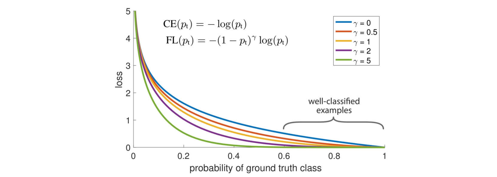
为了更好地控制损失函数的形状,额外引入一个权重系数$\alpha$。
\[FocalLoss(p_t) = -\alpha(1-p_t)^\gamma \log p_t\]
实验中取$\alpha=0.25, \gamma=2$。
def calc_iou(a, b):
    max_length = torch.max(a)
    a = a / max_length
    b = b / max_length

    area = (b[:, 2] - b[:, 0]) * (b[:, 3] - b[:, 1])
    iw = torch.min(torch.unsqueeze(a[:, 3], dim=1), b[:, 2]) - torch.max(torch.unsqueeze(a[:, 1], 1), b[:, 0])
    ih = torch.min(torch.unsqueeze(a[:, 2], dim=1), b[:, 3]) - torch.max(torch.unsqueeze(a[:, 0], 1), b[:, 1])
    iw = torch.clamp(iw, min=0)
    ih = torch.clamp(ih, min=0)
    ua = torch.unsqueeze((a[:, 2] - a[:, 0]) * (a[:, 3] - a[:, 1]), dim=1) + area - iw * ih
    ua = torch.clamp(ua, min=1e-8)
    intersection = iw * ih
    IoU = intersection / ua
    return IoU

def get_target(anchor, bbox_annotation, classification, cuda):
    #   计算真实框和先验框的交并比
    #   anchor              num_anchors, 4
    #   bbox_annotation     num_true_boxes, 5
    #   Iou                 num_anchors, num_true_boxes
    IoU = calc_iou(anchor[:, :], bbox_annotation[:, :4])

    #   计算与先验框重合度最大的真实框
    #   IoU_max             num_anchors,
    #   IoU_argmax          num_anchors,
    IoU_max, IoU_argmax = torch.max(IoU, dim=1)

    #   寻找哪些先验框在计算loss的时候需要忽略
    targets = torch.ones_like(classification) * -1
    targets = targets.type_as(classification)

    #   重合度小于0.4是负样本,需要参与训练
    targets[torch.lt(IoU_max, 0.4), :] = 0

    #   重合度大于0.5是正样本,需要参与训练,还需要计算回归loss
    positive_indices = torch.ge(IoU_max, 0.5)

    #   取出每个先验框最对应的真实框
    assigned_annotations = bbox_annotation[IoU_argmax, :]

    #   将对应的种类置为1
    targets[positive_indices, :] = 0
    targets[positive_indices, assigned_annotations[positive_indices, 4].long()] = 1

    #   计算正样本数量
    num_positive_anchors = positive_indices.sum()
    return targets, num_positive_anchors, positive_indices, assigned_annotations

def encode_bbox(assigned_annotations, positive_indices, anchor_widths, anchor_heights, anchor_ctr_x, anchor_ctr_y):
    #   取出作为正样本的先验框对应的真实框
    assigned_annotations = assigned_annotations[positive_indices, :]

    #   取出作为正样本的先验框
    anchor_widths_pi = anchor_widths[positive_indices]
    anchor_heights_pi = anchor_heights[positive_indices]
    anchor_ctr_x_pi = anchor_ctr_x[positive_indices]
    anchor_ctr_y_pi = anchor_ctr_y[positive_indices]

    #   计算真实框的宽高与中心
    gt_widths = assigned_annotations[:, 2] - assigned_annotations[:, 0]
    gt_heights = assigned_annotations[:, 3] - assigned_annotations[:, 1]
    gt_ctr_x = assigned_annotations[:, 0] + 0.5 * gt_widths
    gt_ctr_y = assigned_annotations[:, 1] + 0.5 * gt_heights

    gt_widths = torch.clamp(gt_widths, min=1)
    gt_heights = torch.clamp(gt_heights, min=1)

    #   利用真实框和先验框进行编码,获得应该有的预测结果
    targets_dx = (gt_ctr_x - anchor_ctr_x_pi) / anchor_widths_pi
    targets_dy = (gt_ctr_y - anchor_ctr_y_pi) / anchor_heights_pi
    targets_dw = torch.log(gt_widths / anchor_widths_pi)
    targets_dh = torch.log(gt_heights / anchor_heights_pi)

    targets = torch.stack((targets_dy, targets_dx, targets_dh, targets_dw))
    targets = targets.t()
    return targets

class FocalLoss(nn.Module):
    def __init__(self):
        super(FocalLoss, self).__init__()

    def forward(self, classifications, regressions, anchors, annotations, alpha = 0.25, gamma = 2.0, cuda = True):
        #   获得batch_size的大小
        batch_size = classifications.shape[0]

        #   获得先验框
        dtype = regressions.dtype
        anchor = anchors[0, :, :].to(dtype)
        #   将先验框转换成中心,宽高的形式
        anchor_widths = anchor[:, 3] - anchor[:, 1]
        anchor_heights = anchor[:, 2] - anchor[:, 0]
        anchor_ctr_x = anchor[:, 1] + 0.5 * anchor_widths
        anchor_ctr_y = anchor[:, 0] + 0.5 * anchor_heights

        regression_losses = []
        classification_losses = []
        for j in range(batch_size):
            #   取出每张图片对应的真实框、种类预测结果和回归预测结果
            bbox_annotation = annotations[j]
            classification = classifications[j, :, :]
            regression = regressions[j, :, :]

            classification = torch.clamp(classification, 5e-4, 1.0 - 5e-4)

            if len(bbox_annotation) == 0:
                #   当图片中不存在真实框的时候,所有特征点均为负样本
                alpha_factor = torch.ones_like(classification) * alpha
                alpha_factor = alpha_factor.type_as(classification)

                alpha_factor = 1. - alpha_factor
                focal_weight = classification
                focal_weight = alpha_factor * torch.pow(focal_weight, gamma)

                #   计算特征点对应的交叉熵
                bce = - (torch.log(1.0 - classification))
                cls_loss = focal_weight * bce
                classification_losses.append(cls_loss.sum())

                #   回归损失此时为0
                regression_losses.append(torch.tensor(0).type_as(classification))
                continue

            #   计算真实框和先验框的交并比
            #   targets                 num_anchors, num_classes
            #   num_positive_anchors    正样本的数量
            #   positive_indices        num_anchors,
            #   assigned_annotations    num_anchors, 5
            targets, num_positive_anchors, positive_indices, assigned_annotations = get_target(anchor,
                                                                                        bbox_annotation, classification, cuda)

            #   首先计算交叉熵loss:focal loss
            alpha_factor = torch.ones_like(targets) * alpha
            alpha_factor = alpha_factor.type_as(classification)
            alpha_factor = torch.where(torch.eq(targets, 1.), alpha_factor, 1. - alpha_factor)
            focal_weight = torch.where(torch.eq(targets, 1.), 1. - classification, classification)
            focal_weight = alpha_factor * torch.pow(focal_weight, gamma)

            bce = - (targets * torch.log(classification) + (1.0 - targets) * torch.log(1.0 - classification))
            cls_loss = focal_weight * bce

            #   把忽略的先验框的loss置为0
            zeros = torch.zeros_like(cls_loss)
            zeros = zeros.type_as(cls_loss)
            cls_loss = torch.where(torch.ne(targets, -1.0), cls_loss, zeros)

            classification_losses.append(cls_loss.sum() / torch.clamp(num_positive_anchors.to(dtype), min=1.0))

            #   如果存在先验框为正样本的话
            if positive_indices.sum() > 0:
                targets = encode_bbox(assigned_annotations, positive_indices, anchor_widths, anchor_heights, anchor_ctr_x, anchor_ctr_y)
                #   将网络应该有的预测结果和实际的预测结果进行比较,计算smooth l1 loss
                regression_diff = torch.abs(targets - regression[positive_indices, :])
                regression_loss = torch.where(
                    torch.le(regression_diff, 1.0 / 9.0),
                    0.5 * 9.0 * torch.pow(regression_diff, 2),
                    regression_diff - 0.5 / 9.0
                )
                regression_losses.append(regression_loss.mean())
            else:
                regression_losses.append(torch.tensor(0).type_as(classification))

        # 计算平均loss并返回
        c_loss = torch.stack(classification_losses).mean()
        r_loss = torch.stack(regression_losses).mean()
        loss = c_loss + r_loss
        return loss, c_loss, r_loss
2. Feature Pyramid Network
RetinaNet的特征提取网络是Feature Pyramid Network (FPN)。FPN提供了具有不同尺度的图像特征,从而可以在不同尺度下检测不同大小的目标。
FPN的结构如图所示。基础结构包含一个金字塔层级序列,每个层级包含多个具有相同尺寸的卷积层和一个$2\times$下采样层。

FPN具有两条路径:
- 自底向上的路径(bottom-up pathway):执行标准的前向传播计算。
- 自顶向下的路径(top-down pathway):把空间分辨率低但是包含更强语义信息的特征增加到前一级输出特征中。
- 首先对高层特征进行$2\times$上采样,采样方法选用最近邻插值;
- 对对应的前向特征使用$1\times 1$卷积减小通道数;
- 将两个特征通过逐元素相加融合。
上述横向连接只发生在每个阶段的输出层特征,对这些融合后的特征使用$3\times 3$卷积处理,并用于后续的目标检测任务中。
根据消融实验,FPN结构的重要性排名为:$1\times 1$横向连接$>$通过多层进行检测$>$自顶向下的增强$>$特征金字塔表示。
class PyramidFeatures(nn.Module):
    def __init__(self, C3_size, C4_size, C5_size, feature_size=256):
        super(PyramidFeatures, self).__init__()

        self.P5_1 = nn.Conv2d(C5_size, feature_size, kernel_size=1, stride=1, padding=0)
        self.P5_2 = nn.Conv2d(feature_size, feature_size, kernel_size=3, stride=1, padding=1)

        self.P4_1 = nn.Conv2d(C4_size, feature_size, kernel_size=1, stride=1, padding=0)
        self.P4_2 = nn.Conv2d(feature_size, feature_size, kernel_size=3, stride=1, padding=1)

        self.P3_1 = nn.Conv2d(C3_size, feature_size, kernel_size=1, stride=1, padding=0)
        self.P3_2 = nn.Conv2d(feature_size, feature_size, kernel_size=3, stride=1, padding=1)

        self.P6 = nn.Conv2d(C5_size, feature_size, kernel_size=3, stride=2, padding=1)

        self.P7_1 = nn.ReLU()
        self.P7_2 = nn.Conv2d(feature_size, feature_size, kernel_size=3, stride=2, padding=1)

    def forward(self, inputs):
        C3, C4, C5 = inputs
        _, _, h4, w4 = C4.size()
        _, _, h3, w3 = C3.size()

        # 75,75,512 -> 75,75,256
        P3_x = self.P3_1(C3)
        # 38,38,1024 -> 38,38,256
        P4_x = self.P4_1(C4)
        # 19,19,2048 -> 19,19,256
        P5_x = self.P5_1(C5)

        # 19,19,256 -> 38,38,256
        P5_upsampled_x = F.interpolate(P5_x, size=(h4, w4))
        # 38,38,256 + 38,38,256 -> 38,38,256
        P4_x = P5_upsampled_x + P4_x
        # 38,38,256 -> 75,75,256
        P4_upsampled_x = F.interpolate(P4_x, size=(h3, w3))
        # 75,75,256 + 75,75,256 -> 75,75,256
        P3_x = P3_x + P4_upsampled_x

        # 75,75,256 -> 75,75,256
        P3_x = self.P3_2(P3_x)
        # 38,38,256 -> 38,38,256
        P4_x = self.P4_2(P4_x)
        # 19,19,256 -> 19,19,256
        P5_x = self.P5_2(P5_x)

        # 19,19,2048 -> 10,10,256
        P6_x = self.P6(C5)

        P7_x = self.P7_1(P6_x)
        # 10,10,256 -> 5,5,256
        P7_x = self.P7_2(P7_x)

        return [P3_x, P4_x, P5_x, P6_x, P7_x]
3. 模型结构
RetinaNet的FPN是基于ResNet构造的。ResNet共有五个层级,每个层级的特征尺寸都是上一层的$1/2$。记第$i$个层级的输出特征是$C_i$,RetinaNet一共使用了$5$个特征金字塔层级,更深的层级能够检测更大的目标:
- $P_3,P_4,P_5$是由ResNet的最后三个层级特征$C_3,C_4,C_5$通过RPN构造的。
- $P_6$是通过对$C_5$应用步长为$2$的$3\times 3$卷积构造的。
- $P_7$是通过对$P_6$应用ReLU和步长为$2$的$3\times 3$卷积构造的。
由于所有层级的输出特征共享后续的分类和回归网络,因此它们具有相同的特征通道数$256$。在每个层级特征上设置$A=9$个anchor:
- $P_3-P_7$的基础边界框尺寸为$32^2-512^2$,设置三种尺寸比例\(\{2^0,2^{1/3},2^{2/3}\}\)。
- 对每个尺寸设置三个长宽比\(\{1/2,1,2\}\)。
对于每个anchor边界框,模型输出$K$个类别的类别概率,并在分类损失上应用focal loss;同时输出边界框位置的回归结果。

class RegressionModel(nn.Module):
    def __init__(self, num_features_in, num_anchors=9, feature_size=256):
        super(RegressionModel, self).__init__()

        self.conv1  = nn.Conv2d(num_features_in, feature_size, kernel_size=3, padding=1)
        self.act1   = nn.ReLU()

        self.conv2  = nn.Conv2d(feature_size, feature_size, kernel_size=3, padding=1)
        self.act2   = nn.ReLU()

        self.conv3  = nn.Conv2d(feature_size, feature_size, kernel_size=3, padding=1)
        self.act3   = nn.ReLU()

        self.conv4  = nn.Conv2d(feature_size, feature_size, kernel_size=3, padding=1)
        self.act4   = nn.ReLU()

        self.output = nn.Conv2d(feature_size, num_anchors * 4, kernel_size=3, padding=1)

    def forward(self, x):
        out = self.conv1(x)
        out = self.act1(out)

        out = self.conv2(out)
        out = self.act2(out)

        out = self.conv3(out)
        out = self.act3(out)

        out = self.conv4(out)
        out = self.act4(out)

        out = self.output(out)

        out = out.permute(0, 2, 3, 1)

        return out.contiguous().view(out.shape[0], -1, 4)

class ClassificationModel(nn.Module):
    def __init__(self, num_features_in, num_anchors=9, num_classes=80, feature_size=256):
        super(ClassificationModel, self).__init__()

        self.num_classes = num_classes
        self.num_anchors = num_anchors

        self.conv1  = nn.Conv2d(num_features_in, feature_size, kernel_size=3, padding=1)
        self.act1   = nn.ReLU()

        self.conv2  = nn.Conv2d(feature_size, feature_size, kernel_size=3, padding=1)
        self.act2   = nn.ReLU()

        self.conv3  = nn.Conv2d(feature_size, feature_size, kernel_size=3, padding=1)
        self.act3   = nn.ReLU()

        self.conv4  = nn.Conv2d(feature_size, feature_size, kernel_size=3, padding=1)
        self.act4   = nn.ReLU()

        self.output = nn.Conv2d(feature_size, num_anchors * num_classes, kernel_size=3, padding=1)
        self.output_act = nn.Sigmoid()

    def forward(self, x):
        out = self.conv1(x)
        out = self.act1(out)

        out = self.conv2(out)
        out = self.act2(out)

        out = self.conv3(out)
        out = self.act3(out)

        out = self.conv4(out)
        out = self.act4(out)

        out = self.output(out)
        out = self.output_act(out)

        # out is B x C x W x H, with C = n_classes * n_anchors
        out1 = out.permute(0, 2, 3, 1)

        batch_size, height, width, channels = out1.shape

        out2 = out1.view(batch_size, height, width, self.num_anchors, self.num_classes)

        return out2.contiguous().view(x.shape[0], -1, self.num_classes)

class Resnet(nn.Module):
    def __init__(self, phi, pretrained=False):
        super(Resnet, self).__init__()
        self.edition = [resnet18, resnet34, resnet50, resnet101, resnet152]
        model = self.edition[phi](pretrained)
        del model.avgpool
        del model.fc
        self.model = model

    def forward(self, x):
        x = self.model.conv1(x)
        x = self.model.bn1(x)
        x = self.model.relu(x)
        x = self.model.maxpool(x)

        x = self.model.layer1(x)
        feat1 = self.model.layer2(x)
        feat2 = self.model.layer3(feat1)
        feat3 = self.model.layer4(feat2)

        return [feat1,feat2,feat3]

class retinanet(nn.Module):
    def __init__(self, num_classes, phi, pretrained=False, fp16=False):
        super(retinanet, self).__init__()
        self.pretrained = pretrained
        self.backbone_net = Resnet(phi, pretrained)
        fpn_sizes = {
            0: [128, 256, 512],
            1: [128, 256, 512],
            2: [512, 1024, 2048],
            3: [512, 1024, 2048],
            4: [512, 1024, 2048],
        }[phi]

        self.fpn = PyramidFeatures(fpn_sizes[0], fpn_sizes[1], fpn_sizes[2])

        self.regressionModel        = RegressionModel(256)
        self.classificationModel    = ClassificationModel(256, num_classes=num_classes)
        self.anchors = Anchors()

    def forward(self, inputs):
        #   取出三个有效特征层,分别是C3、C4、C5
        #   假设输入图像为600,600,3
        #   当我们使用resnet50的时候
        #   C3     75,75,512
        #   C4     38,38,1024
        #   C5     19,19,2048
        p3, p4, p5 = self.backbone_net(inputs)

        #   经过FPN可以获得5个有效特征层分别是
        #   P3     75,75,256
        #   P4     38,38,256
        #   P5     19,19,256
        #   P6     10,10,256
        #   P7     5,5,256
        features = self.fpn([p3, p4, p5])

        #   将获取到的P3, P4, P5, P6, P7传入到
        #   Retinahead里面进行预测,获得回归预测结果和分类预测结果
        #   将所有特征层的预测结果进行堆叠
        regression      = torch.cat([self.regressionModel(feature) for feature in features], dim=1)
        classification  = torch.cat([self.classificationModel(feature) for feature in features], dim=1)

        anchors = self.anchors(features)

        return features, regression, classification, anchors
RetinaNet的完整PyTorch实现可参考 retinanet-pytorch。

